pacman::p_load(sf, spdep, tmap, tidyverse)Handon_Ex07
Local Measures of Spatial Autocorrelation
Overview
Learn compute Global and Local Measure of Spatial Autocorrelation (GLSA) by using spdep package
Getting Started
The analytical question
In spatial policy, one of the main development objective of the local govenment and planners is to ensure equal distribution of development in the province. Our task in this study, hence, is to apply appropriate spatial statistical methods to discover if development are even distributed geographically. If the answer is No. Then, our next question will be “is there sign of spatial clustering?”. And, if the answer for this question is yes, then our next question will be “where are these clusters?
The Study Area and Data
Two data sets will be used in this hands-on exercise, they are:
Hunan province administrative boundary layer at county level. This is a geospatial data set in ESRI shapefile format.
Hunan_2012.csv: This csv file contains selected Hunan’s local development indicators in 2012.
Setting the Analytical Toolls
Before we get started, we need to ensure that spdep, sf, tmap and tidyverse packages of R are currently installed in your R.
sf is use for importing and handling geospatial data in R,
tidyverse is mainly use for wrangling attribute data in R,
spdep will be used to compute spatial weights, global and local spatial autocorrelation statistics, and
tmap will be used to prepare cartographic quality chropleth map.
Getting the Data Into R Environment
hunan <- st_read(dsn = "data/geospatial",
                 layer = "Hunan")
Reading layer `Hunan' from data source
`C:\Quanfang777\IS415-GAA\WeeklyExercise\week7\Hands-on_Ex07\data\geospatial'
using driver `ESRI Shapefile'
Simple feature collection with 88 features and 7 fields
Geometry type: POLYGON
Dimension: XY
Bounding box: xmin: 108.7831 ymin: 24.6342 xmax: 114.2544 ymax: 30.12812
Geodetic CRS: WGS 84hunan2012 <- read_csv("data/aspatial/Hunan_2012.csv")Rows: 88 Columns: 29
── Column specification ────────────────────────────────────────────────────────
Delimiter: ","
chr (2): County, City
dbl (27): avg_wage, deposite, FAI, Gov_Rev, Gov_Exp, GDP, GDPPC, GIO, Loan, ...
ℹ Use `spec()` to retrieve the full column specification for this data.
ℹ Specify the column types or set `show_col_types = FALSE` to quiet this message.Performing relational join
hunan <- left_join(hunan,hunan2012) %>%
  select(1:4, 7, 15)
Joining, by = "County"equal <- tm_shape(hunan) +
tm_fill("GDPPC",
n = 5,
style = "equal") +
tm_borders(alpha = 0.5) +
tm_layout(main.title = "Equal interval classification")
quantile <- tm_shape(hunan) +
tm_fill("GDPPC",
n = 5,
style = "quantile") +
tm_borders(alpha = 0.5) +
tm_layout(main.title = "Equal quantile classification")
tmap_arrange(equal,
quantile,
asp=1,
ncol=2)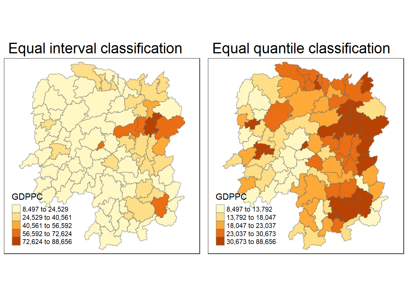
Global Spatial Autocorrelation
Learn how to compute global spatial autocorrelation statistics and to perform spatial complete randomness test for global spatial autocorrelation.
Computing Contiguity Spatial Weights
Before we can compute the global spatial autocorrelation statistics, we need to construct a spatial weights of the study area. The spatial weights is used to define the neighbourhood relationships between the geographical units (i.e. county) in the study area.
In the code chunk below, poly2nb() of spdep package is used to compute contiguity weight matrices for the study area. This function builds a neighbours list based on regions with contiguous boundaries. If you look at the documentation you will see that you can pass a “queen” argument that takes TRUE or FALSE as options. If you do not specify this argument the default is set to TRUE, that is, if you don’t specify queen = FALSE this function will return a list of first order neighbours using the Queen criteria.
wm_q <- poly2nb(hunan,
                queen=TRUE)
summary(wm_q)
Neighbour list object:
Number of regions: 88
Number of nonzero links: 448
Percentage nonzero weights: 5.785124
Average number of links: 5.090909
Link number distribution:
1 2 3 4 5 6 7 8 9 11
2 2 12 16 24 14 11 4 2 1
2 least connected regions:
30 65 with 1 link
1 most connected region:
85 with 11 linksThe summary report above shows that there are 88 area units in Hunan. The most connected area unit has 11 neighbours. There are two area units with only one neighbours.
Row-standardised weights matrix
rswm_q <- nb2listw(wm_q,
                   style="W",
                   zero.policy = TRUE)
rswm_q
Characteristics of weights list object:
Neighbour list object:
Number of regions: 88
Number of nonzero links: 448
Percentage nonzero weights: 5.785124
Average number of links: 5.090909
Weights style: W
Weights constants summary:
n nn S0 S1 S2
W 88 7744 88 37.86334 365.9147Global Spatial Autocorrelation: Moran’s I
The code chunk below performs Moran’s I statistical testing using moran.test() of spdep.
moran.test(hunan$GDPPC,
           listw=rswm_q,
           zero.policy = TRUE,
           na.action=na.omit)
    Moran I test under randomisation

data:  hunan$GDPPC
weights: rswm_q

Moran I statistic standard deviate = 4.7351, p-value = 1.095e-06
alternative hypothesis: greater
sample estimates:
Moran I statistic       Expectation          Variance
      0.300749970      -0.011494253       0.004348351
Computing Monte Carlo Moran’s I
set.seed(1234)
bperm= moran.mc(hunan$GDPPC,
                listw=rswm_q,
                nsim=999,
                zero.policy = TRUE,
                na.action=na.omit)
bperm
    Monte-Carlo simulation of Moran I

data:  hunan$GDPPC
weights: rswm_q
number of simulations + 1: 1000

statistic = 0.30075, observed rank = 1000, p-value = 0.001
alternative hypothesis: greater
Visualising Monte Carlo Moran’s I
hist(bperm$res,
     freq=TRUE,
     breaks=20,
     xlab="Simulated Moran's I")
abline(v=0,
       col="red")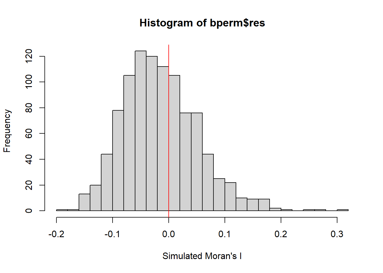
Global Spatial Autocorrelation: Geary’s
Learn how to perform Geary’s c statistics testing by using appropriate functions of spdep package
geary.test(hunan$GDPPC, listw=rswm_q)
    Geary C test under randomisation

data:  hunan$GDPPC
weights: rswm_q

Geary C statistic standard deviate = 3.6108, p-value = 0.0001526
alternative hypothesis: Expectation greater than statistic
sample estimates:
Geary C statistic       Expectation          Variance
        0.6907223         1.0000000         0.0073364
Computing Monte Carlo Geary’s C
set.seed(1234)
bperm=geary.mc(hunan$GDPPC,
               listw=rswm_q,
               nsim=999)
bperm
    Monte-Carlo simulation of Geary C

data:  hunan$GDPPC
weights: rswm_q
number of simulations + 1: 1000

statistic = 0.69072, observed rank = 1, p-value = 0.001
alternative hypothesis: greater
Visualising the Monte Carlo Geary’s C
hist(bperm$res, freq=TRUE, breaks=20, xlab="Simulated Geary c")
abline(v=1, col="red") 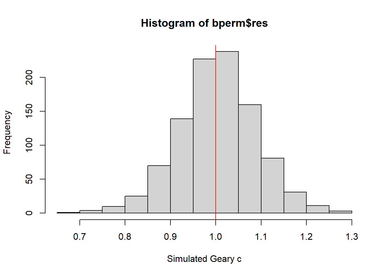
Spatial Correlogram
Spatial correlograms are great to examine patterns of spatial autocorrelation in your data or model residuals. They show how correlated are pairs of spatial observations when you increase the distance (lag) between them - they are plots of some index of autocorrelation (Moran’s I or Geary’s c) against distance.Although correlograms are not as fundamental as variograms (a keystone concept of geostatistics), they are very useful as an exploratory and descriptive tool. For this purpose they actually provide richer information than variograms.
Compute Moran’s I correlogram
MI_corr <- sp.correlogram(wm_q,
                          hunan$GDPPC,
                          order=6,
                          method="I",
                          style="W")
plot(MI_corr)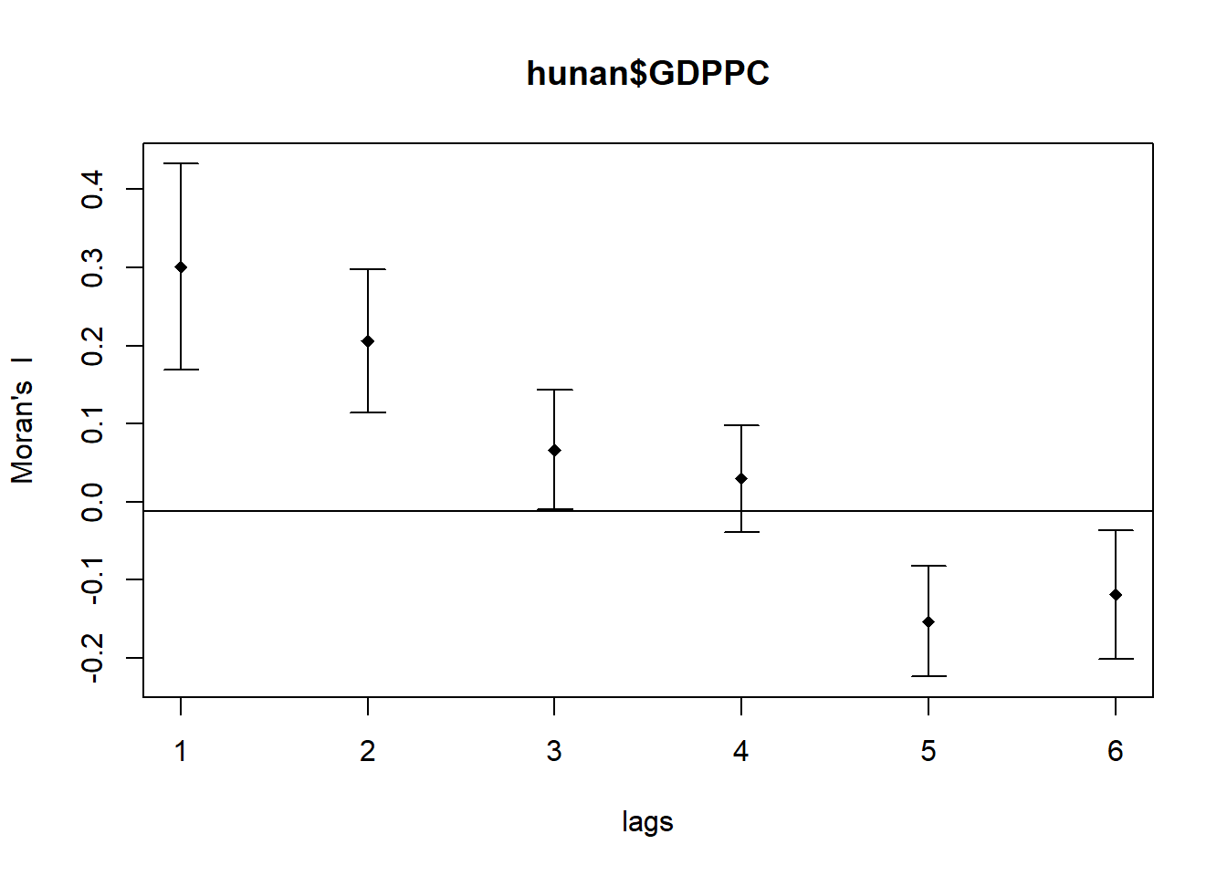
print(MI_corr)Spatial correlogram for hunan$GDPPC
method: Moran's I
estimate expectation variance standard deviate Pr(I) two sided
1 (88) 0.3007500 -0.0114943 0.0043484 4.7351 2.189e-06 ***
2 (88) 0.2060084 -0.0114943 0.0020962 4.7505 2.029e-06 ***
3 (88) 0.0668273 -0.0114943 0.0014602 2.0496 0.040400 *
4 (88) 0.0299470 -0.0114943 0.0011717 1.2107 0.226015
5 (88) -0.1530471 -0.0114943 0.0012440 -4.0134 5.984e-05 ***
6 (88) -0.1187070 -0.0114943 0.0016791 -2.6164 0.008886 **
---
Signif. codes: 0 '***' 0.001 '**' 0.01 '*' 0.05 '.' 0.1 ' ' 1Compute Geary’s C correlogram and plot
In the code chunk below, sp.correlogram() of spdep package is used to compute a 6-lag spatial correlogram of GDPPC. The global spatial autocorrelation used in Geary’s C. The plot() of base Graph is then used to plot the output.
GC_corr <- sp.correlogram(wm_q,
                          hunan$GDPPC,
                          order=6,
                          method="C",
                          style="W")
plot(GC_corr)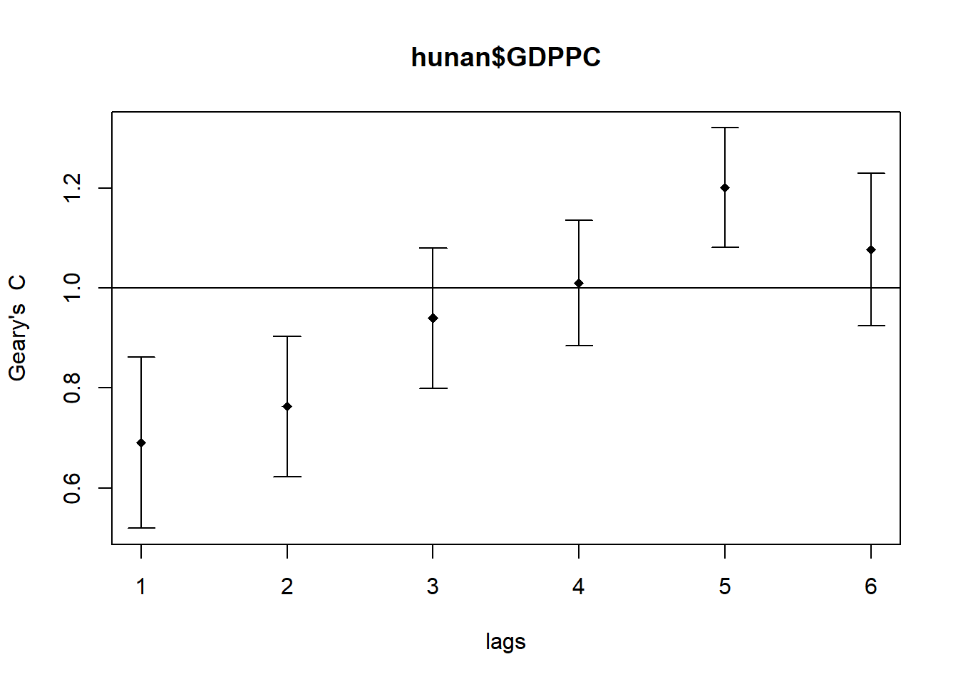
print(GC_corr)Spatial correlogram for hunan$GDPPC
method: Geary's C
estimate expectation variance standard deviate Pr(I) two sided
1 (88) 0.6907223 1.0000000 0.0073364 -3.6108 0.0003052 ***
2 (88) 0.7630197 1.0000000 0.0049126 -3.3811 0.0007220 ***
3 (88) 0.9397299 1.0000000 0.0049005 -0.8610 0.3892612
4 (88) 1.0098462 1.0000000 0.0039631 0.1564 0.8757128
5 (88) 1.2008204 1.0000000 0.0035568 3.3673 0.0007592 ***
6 (88) 1.0773386 1.0000000 0.0058042 1.0151 0.3100407
---
Signif. codes: 0 '***' 0.001 '**' 0.01 '*' 0.05 '.' 0.1 ' ' 1Cluster and Outlier Analysis
Local Indicators of Spatial Association or LISA are statistics that evaluate the existence of clusters in the spatial arrangement of a given variable. For instance if we are studying cancer rates among census tracts in a given city local clusters in the rates mean that there are areas that have higher or lower rates than is to be expected by chance alone; that is, the values occurring are above or below those of a random distribution in space.
In this section will illustrate how to apply appropriate Local Indicators for Spatial Association (LISA), especially local Moran’I to detect cluster and/or outlier from GDP per capita 2012 of Hunan Province, PRC.
Computing local Moran’s I To compute local Moran’s I, the localmoran() function of spdep will be used. It computes Ii values, given a set of zi values and a listw object providing neighbour weighting information for the polygon associated with the zi values.
The code chunks below are used to compute local Moran’s I of GDPPC2012 at the county level.
fips <- order(hunan$County)
localMI <- localmoran(hunan$GDPPC, rswm_q)
head(localMI)
Ii E.Ii Var.Ii Z.Ii Pr(z != E(Ii))
1 -0.001468468 -2.815006e-05 4.723841e-04 -0.06626904 0.9471636
2 0.025878173 -6.061953e-04 1.016664e-02 0.26266425 0.7928094
3 -0.011987646 -5.366648e-03 1.133362e-01 -0.01966705 0.9843090
4 0.001022468 -2.404783e-07 5.105969e-06 0.45259801 0.6508382
5 0.014814881 -6.829362e-05 1.449949e-03 0.39085814 0.6959021
6 -0.038793829 -3.860263e-04 6.475559e-03 -0.47728835 0.6331568ocalmoran() function returns a matrix of values whose columns are:
Ii: the local Moran’s I statistics
E.Ii: the expectation of local moran statistic under the randomisation hypothesis
Var.Ii: the variance of local moran statistic under the randomisation hypothesis
Z.Ii:the standard deviate of local moran statistic
Pr(): the p-value of local moran statistic
The code chunk below list the content of the local Moran matrix derived by using printCoefmat().
printCoefmat(data.frame(
  localMI[fips,],
  row.names=hunan$County[fips]),
  check.names=FALSE)
Ii E.Ii Var.Ii Z.Ii Pr.z....E.Ii..
Anhua -2.2493e-02 -5.0048e-03 5.8235e-02 -7.2467e-02 0.9422
Anren -3.9932e-01 -7.0111e-03 7.0348e-02 -1.4791e+00 0.1391
Anxiang -1.4685e-03 -2.8150e-05 4.7238e-04 -6.6269e-02 0.9472
Baojing 3.4737e-01 -5.0089e-03 8.3636e-02 1.2185e+00 0.2230
Chaling 2.0559e-02 -9.6812e-04 2.7711e-02 1.2932e-01 0.8971
Changning -2.9868e-05 -9.0010e-09 1.5105e-07 -7.6828e-02 0.9388
Changsha 4.9022e+00 -2.1348e-01 2.3194e+00 3.3590e+00 0.0008
Chengbu 7.3725e-01 -1.0534e-02 2.2132e-01 1.5895e+00 0.1119
Chenxi 1.4544e-01 -2.8156e-03 4.7116e-02 6.8299e-01 0.4946
Cili 7.3176e-02 -1.6747e-03 4.7902e-02 3.4200e-01 0.7324
Dao 2.1420e-01 -2.0824e-03 4.4123e-02 1.0297e+00 0.3032
Dongan 1.5210e-01 -6.3485e-04 1.3471e-02 1.3159e+00 0.1882
Dongkou 5.2918e-01 -6.4461e-03 1.0748e-01 1.6338e+00 0.1023
Fenghuang 1.8013e-01 -6.2832e-03 1.3257e-01 5.1198e-01 0.6087
Guidong -5.9160e-01 -1.3086e-02 3.7003e-01 -9.5104e-01 0.3416
Guiyang 1.8240e-01 -3.6908e-03 3.2610e-02 1.0305e+00 0.3028
Guzhang 2.8466e-01 -8.5054e-03 1.4152e-01 7.7931e-01 0.4358
Hanshou 2.5878e-02 -6.0620e-04 1.0167e-02 2.6266e-01 0.7928
Hengdong 9.9964e-03 -4.9063e-04 6.7742e-03 1.2742e-01 0.8986
Hengnan 2.8064e-02 -3.2160e-04 3.7597e-03 4.6294e-01 0.6434
Hengshan -5.8201e-03 -3.0437e-05 5.1076e-04 -2.5618e-01 0.7978
Hengyang 6.2997e-02 -1.3046e-03 2.1865e-02 4.3486e-01 0.6637
Hongjiang 1.8790e-01 -2.3019e-03 3.1725e-02 1.0678e+00 0.2856
Huarong -1.5389e-02 -1.8667e-03 8.1030e-02 -4.7503e-02 0.9621
Huayuan 8.3772e-02 -8.5569e-04 2.4495e-02 5.4072e-01 0.5887
Huitong 2.5997e-01 -5.2447e-03 1.1077e-01 7.9685e-01 0.4255
Jiahe -1.2431e-01 -3.0550e-03 5.1111e-02 -5.3633e-01 0.5917
Jianghua 2.8651e-01 -3.8280e-03 8.0968e-02 1.0204e+00 0.3076
Jiangyong 2.4337e-01 -2.7082e-03 1.1746e-01 7.1800e-01 0.4728
Jingzhou 1.8270e-01 -8.5106e-04 2.4363e-02 1.1759e+00 0.2396
Jinshi -1.1988e-02 -5.3666e-03 1.1334e-01 -1.9667e-02 0.9843
Jishou -2.8680e-01 -2.6305e-03 4.4028e-02 -1.3543e+00 0.1756
Lanshan 6.3334e-02 -9.6365e-04 2.0441e-02 4.4972e-01 0.6529
Leiyang 1.1581e-02 -1.4948e-04 2.5082e-03 2.3422e-01 0.8148
Lengshuijiang -1.7903e+00 -8.2129e-02 2.1598e+00 -1.1623e+00 0.2451
Li 1.0225e-03 -2.4048e-07 5.1060e-06 4.5260e-01 0.6508
Lianyuan -1.4672e-01 -1.8983e-03 1.9145e-02 -1.0467e+00 0.2952
Liling 1.3774e+00 -1.5097e-02 4.2601e-01 2.1335e+00 0.0329
Linli 1.4815e-02 -6.8294e-05 1.4499e-03 3.9086e-01 0.6959
Linwu -2.4621e-03 -9.0703e-06 1.9258e-04 -1.7676e-01 0.8597
Linxiang 6.5904e-02 -2.9028e-03 2.5470e-01 1.3634e-01 0.8916
Liuyang 3.3688e+00 -7.7502e-02 1.5180e+00 2.7972e+00 0.0052
Longhui 8.0801e-01 -1.1377e-02 1.5538e-01 2.0787e+00 0.0376
Longshan 7.5663e-01 -1.1100e-02 3.1449e-01 1.3690e+00 0.1710
Luxi 1.8177e-01 -2.4855e-03 3.4249e-02 9.9561e-01 0.3194
Mayang 2.1852e-01 -5.8773e-03 9.8049e-02 7.1663e-01 0.4736
Miluo 1.8704e+00 -1.6927e-02 2.7925e-01 3.5715e+00 0.0004
Nan -9.5789e-03 -4.9497e-04 6.8341e-03 -1.0988e-01 0.9125
Ningxiang 1.5607e+00 -7.3878e-02 8.0012e-01 1.8274e+00 0.0676
Ningyuan 2.0910e-01 -7.0884e-03 8.2306e-02 7.5356e-01 0.4511
Pingjiang -9.8964e-01 -2.6457e-03 5.6027e-02 -4.1698e+00 0.0000
Qidong 1.1806e-01 -2.1207e-03 2.4747e-02 7.6396e-01 0.4449
Qiyang 6.1966e-02 -7.3374e-04 8.5743e-03 6.7712e-01 0.4983
Rucheng -3.6992e-01 -8.8999e-03 2.5272e-01 -7.1814e-01 0.4727
Sangzhi 2.5053e-01 -4.9470e-03 6.8000e-02 9.7972e-01 0.3272
Shaodong -3.2659e-02 -3.6592e-05 5.0546e-04 -1.4510e+00 0.1468
Shaoshan 2.1223e+00 -5.0227e-02 1.3668e+00 1.8583e+00 0.0631
Shaoyang 5.9499e-01 -1.1253e-02 1.3012e-01 1.6807e+00 0.0928
Shimen -3.8794e-02 -3.8603e-04 6.4756e-03 -4.7729e-01 0.6332
Shuangfeng 9.2835e-03 -2.2867e-03 3.1516e-02 6.5174e-02 0.9480
Shuangpai 8.0591e-02 -3.1366e-04 8.9838e-03 8.5358e-01 0.3933
Suining 3.7585e-01 -3.5933e-03 4.1870e-02 1.8544e+00 0.0637
Taojiang -2.5394e-01 -1.2395e-03 1.4477e-02 -2.1002e+00 0.0357
Taoyuan 1.4729e-02 -1.2039e-04 8.5103e-04 5.0903e-01 0.6107
Tongdao 4.6482e-01 -6.9870e-03 1.9879e-01 1.0582e+00 0.2900
Wangcheng 4.4220e+00 -1.1067e-01 1.3596e+00 3.8873e+00 0.0001
Wugang 7.1003e-01 -7.8144e-03 1.0710e-01 2.1935e+00 0.0283
Xiangtan 2.4530e-01 -3.6457e-04 3.2319e-03 4.3213e+00 0.0000
Xiangxiang 2.6271e-01 -1.2703e-03 2.1290e-02 1.8092e+00 0.0704
Xiangyin 5.4525e-01 -4.7442e-03 7.9236e-02 1.9539e+00 0.0507
Xinhua 1.1810e-01 -6.2649e-03 8.6001e-02 4.2409e-01 0.6715
Xinhuang 1.5725e-01 -4.1820e-03 3.6648e-01 2.6667e-01 0.7897
Xinning 6.8928e-01 -9.6674e-03 2.0328e-01 1.5502e+00 0.1211
Xinshao 5.7578e-02 -8.5932e-03 1.1769e-01 1.9289e-01 0.8470
Xintian -7.4050e-03 -5.1493e-03 1.0877e-01 -6.8395e-03 0.9945
Xupu 3.2406e-01 -5.7468e-03 5.7735e-02 1.3726e+00 0.1699
Yanling -6.9021e-02 -5.9211e-04 9.9306e-03 -6.8667e-01 0.4923
Yizhang -2.6844e-01 -2.2463e-03 4.7588e-02 -1.2202e+00 0.2224
Yongshun 6.3064e-01 -1.1350e-02 1.8830e-01 1.4795e+00 0.1390
Yongxing 4.3411e-01 -9.0735e-03 1.5088e-01 1.1409e+00 0.2539
You 7.8750e-02 -7.2728e-03 1.2116e-01 2.4714e-01 0.8048
Yuanjiang 2.0004e-04 -1.7760e-04 2.9798e-03 6.9181e-03 0.9945
Yuanling 8.7298e-03 -2.2981e-06 2.3221e-05 1.8121e+00 0.0700
Yueyang 4.1189e-02 -1.9768e-04 2.3113e-03 8.6085e-01 0.3893
Zhijiang 1.0476e-01 -7.8123e-04 1.3100e-02 9.2214e-01 0.3565
Zhongfang -2.2685e-01 -2.1455e-03 3.5927e-02 -1.1855e+00 0.2358
Zhuzhou 3.2864e-01 -5.2432e-04 7.2391e-03 3.8688e+00 0.0001
Zixing -7.6849e-01 -8.8210e-02 9.4057e-01 -7.0144e-01 0.4830Mapping the local Moran’s I
hunan.localMI <- cbind(hunan,localMI) %>%
  rename(Pr.Ii = Pr.z....E.Ii..)
Mapping local Moran’s I values
tm_shape(hunan.localMI) +
  tm_fill(col = "Ii",
          style = "pretty",
          palette = "RdBu",
          title = "local moran statistics") +
  tm_borders(alpha = 0.5)
Variable(s) "Ii" contains positive and negative values, so midpoint is set to 0. Set midpoint = NA to show the full spectrum of the color palette.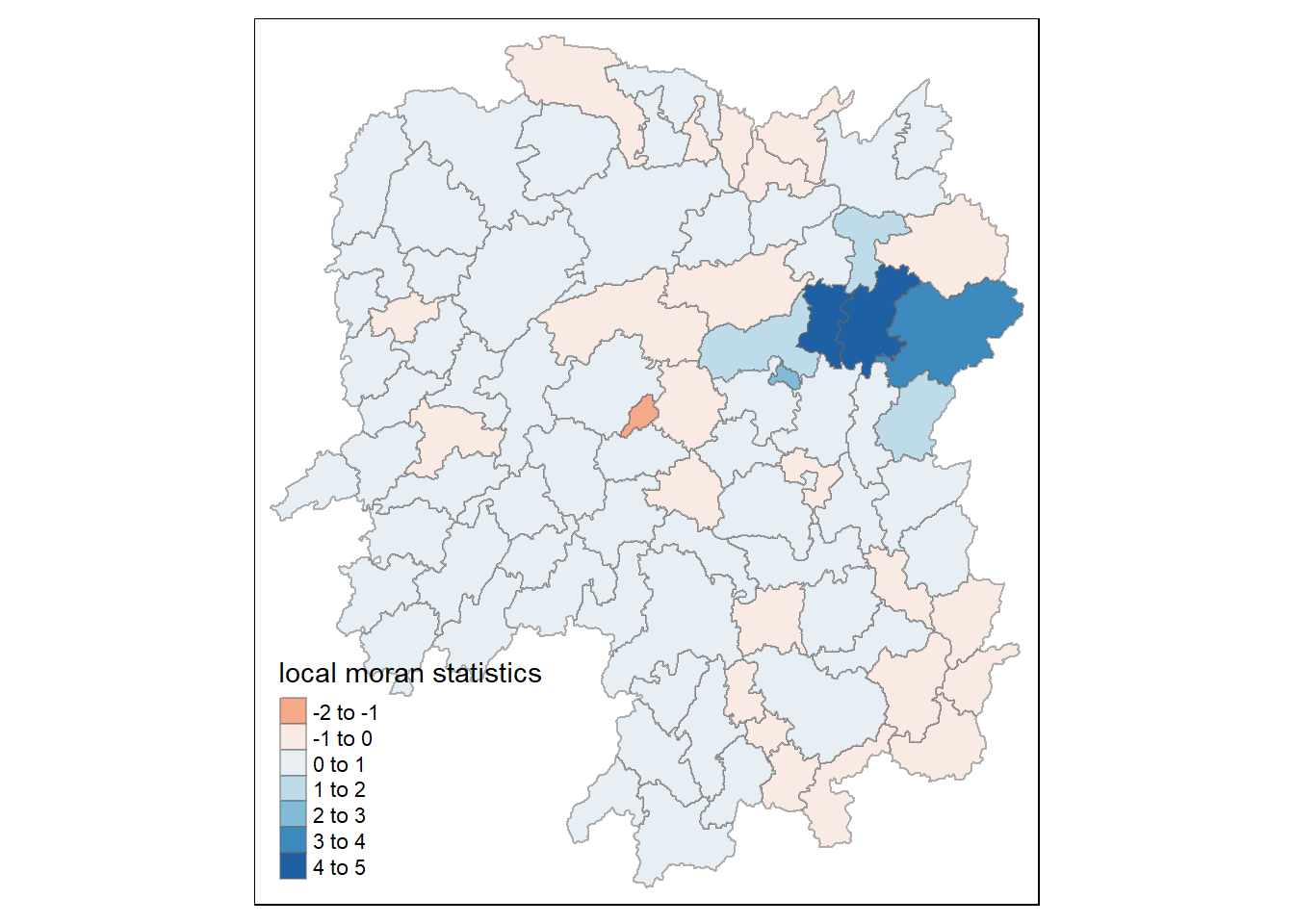
Mapping local Moran’s I p-values
The choropleth shows there is evidence for both positive and negative Ii values. However, it is useful to consider the p-values for each of these values, as consider above.
The code chunks below produce a choropleth map of Moran’s I p-values by using functions of tmap package.
tm_shape(hunan.localMI) +
  tm_fill(col = "Pr.Ii",
          breaks=c(-Inf, 0.001, 0.01, 0.05, 0.1, Inf),
          palette="-Blues",
          title = "local Moran's I p-values") +
  tm_borders(alpha = 0.5)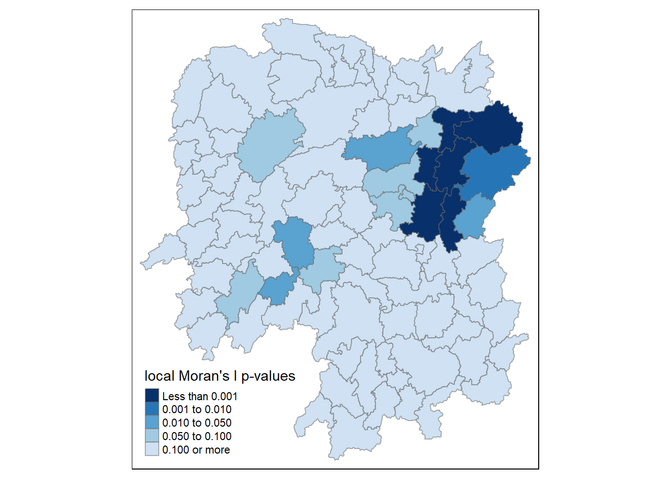
Mapping both local Moran’s I values and p-values
For effective interpretation, it is better to plot both the local Moran’s I values map and its corresponding p-values map next to each other.
The code chunk below will be used to create such visualisation.
localMI.map <- tm_shape(hunan.localMI) +
  tm_fill(col = "Ii",
          style = "pretty",
          title = "local moran statistics") +
  tm_borders(alpha = 0.5)

pvalue.map <- tm_shape(hunan.localMI) +
  tm_fill(col = "Pr.Ii",
          breaks=c(-Inf, 0.001, 0.01, 0.05, 0.1, Inf),
          palette="-Blues",
          title = "local Moran's I p-values") +
  tm_borders(alpha = 0.5)

tmap_arrange(localMI.map, pvalue.map, asp=1, ncol=2)
Variable(s) "Ii" contains positive and negative values, so midpoint is set to 0. Set midpoint = NA to show the full spectrum of the color palette.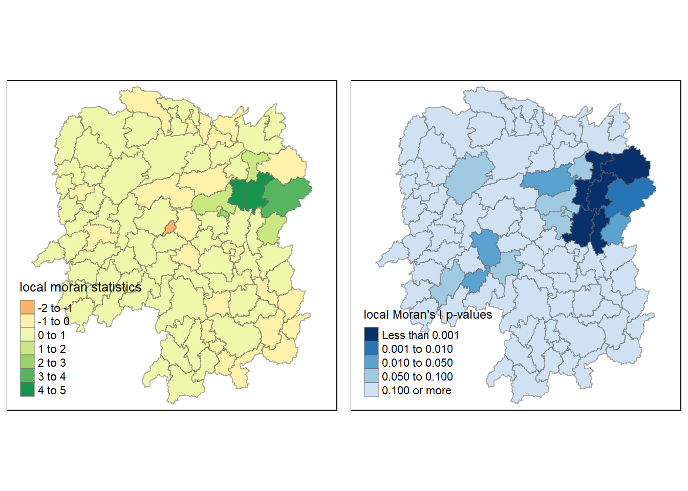
Creating a LISA Cluster Map
The LISA Cluster Map shows the significant locations color coded by type of spatial autocorrelation. The first step before we can generate the LISA cluster map is to plot the Moran scatterplot.
Plotting Moran scatterplot
The Moran scatterplot is an illustration of the relationship between the values of the chosen attribute at each location and the average value of the same attribute at neighboring locations.
The code chunk below plots the Moran scatterplot of GDPPC 2012 by using moran.plot() of spdep.
nci <- moran.plot(hunan$GDPPC, rswm_q,
                  labels=as.character(hunan$County),
                  xlab="GDPPC 2012",
                  ylab="Spatially Lag GDPPC 2012")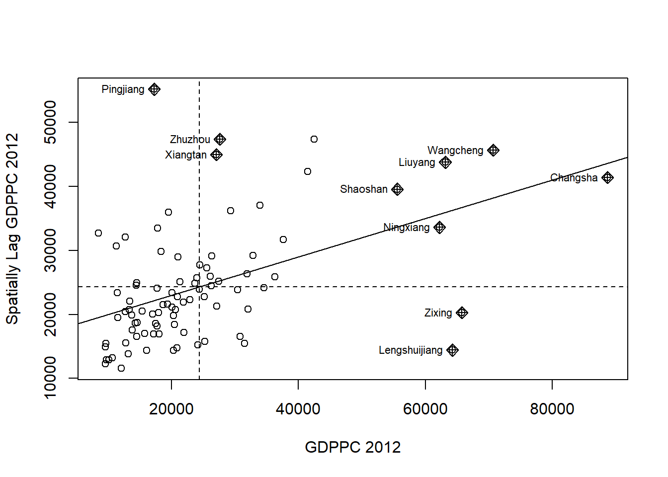
Notice that the plot is split in 4 quadrants. The top right corner belongs to areas that have high GDPPC and are surrounded by other areas that have the average level of GDPPC. This are the high-high locations in the lesson slide.
Plotting Moran scatterplot with standardised variable
First we will use scale() to centers and scales the variable. Here centering is done by subtracting the mean (omitting NAs) the corresponding columns, and scaling is done by dividing the (centered) variable by their standard deviations.
hunan$Z.GDPPC <- scale(hunan$GDPPC) %>%
  as.vector
nci2 <- moran.plot(hunan$Z.GDPPC, rswm_q,
labels=as.character(hunan$County),
xlab="z-GDPPC 2012",
ylab="Spatially Lag z-GDPPC 2012")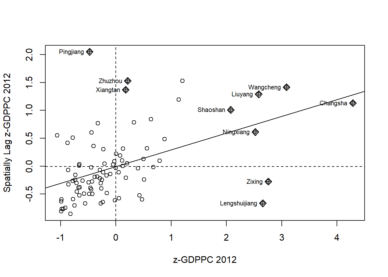
Preparing LISA map classes
quadrant <- vector(mode="numeric",length=nrow(localMI))
hunan$lag_GDPPC <- lag.listw(rswm_q, hunan$GDPPC)
DV <- hunan$lag_GDPPC - mean(hunan$lag_GDPPC)
LM_I <- localMI[,1]
signif <- 0.05
quadrant[DV <0 & LM_I>0] <- 1
quadrant[DV >0 & LM_I<0] <- 2
quadrant[DV <0 & LM_I<0] <- 3
quadrant[DV >0 & LM_I>0] <- 4
quadrant[localMI[,5]>signif] <- 0
Plotting LISA map
hunan.localMI$quadrant <- quadrant
colors <- c("#ffffff", "#2c7bb6", "#abd9e9", "#fdae61", "#d7191c")
clusters <- c("insignificant", "low-low", "low-high", "high-low", "high-high")

tm_shape(hunan.localMI) +
  tm_fill(col = "quadrant",
          style = "cat",
          palette = colors[c(sort(unique(quadrant)))+1],
          labels = clusters[c(sort(unique(quadrant)))+1],
          popup.vars = c("")) +
  tm_view(set.zoom.limits = c(11,17)) +
  tm_borders(alpha=0.5)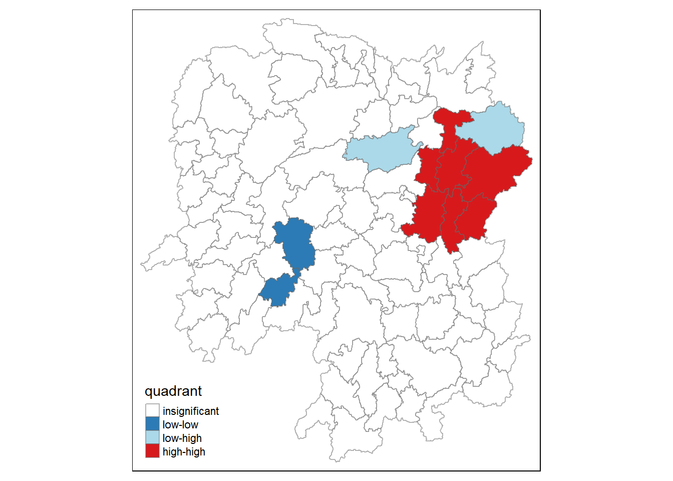
For effective interpretation, it is better to plot both the local Moran’s I values map and its corresponding p-values map next to each other.
The code chunk below will be used to create such visualisation.
gdppc <- qtm(hunan, "GDPPC")

hunan.localMI$quadrant <- quadrant
colors <- c("#ffffff", "#2c7bb6", "#abd9e9", "#fdae61", "#d7191c")
clusters <- c("insignificant", "low-low", "low-high", "high-low", "high-high")

LISAmap <- tm_shape(hunan.localMI) +
  tm_fill(col = "quadrant",
          style = "cat",
          palette = colors[c(sort(unique(quadrant)))+1],
          labels = clusters[c(sort(unique(quadrant)))+1],
          popup.vars = c("")) +
  tm_view(set.zoom.limits = c(11,17)) +
  tm_borders(alpha=0.5)

tmap_arrange(gdppc, LISAmap,
             asp=1, ncol=2)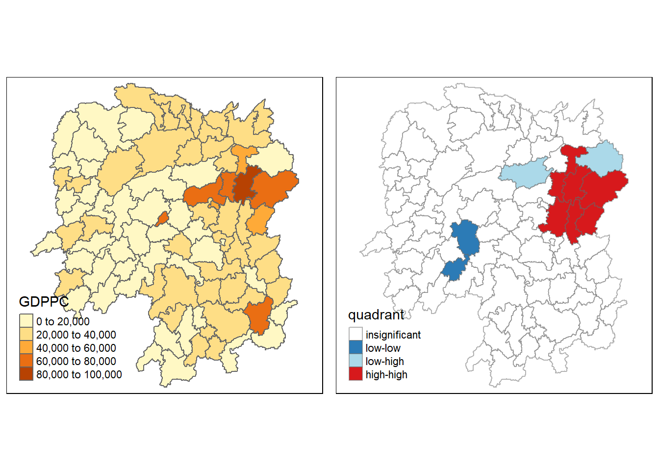
Hot Spot and Cold Spot Area Analysis
Beside detecting cluster and outliers, localised spatial statistics can be also used to detect hot spot and/or cold spot areas.
The term ‘hot spot’ has been used generically across disciplines to describe a region or value that is higher relative to its surroundings (Lepers et al 2005, Aben et al 2012, Isobe et al 2015).
Getis and Ord’s G-Statistics
An alternative spatial statistics to detect spatial anomalies is the Getis and Ord’s G-statistics (Getis and Ord, 1972; Ord and Getis, 1995). It looks at neighbours within a defined proximity to identify where either high or low values clutser spatially. Here, statistically significant hot-spots are recognised as areas of high values where other areas within a neighbourhood range also share high values too.
The analysis consists of three steps:
Deriving spatial weight matrix
Computing Gi statistics
Mapping Gi statistics
Deriving distance-based weight matrix
First, we need to define a new set of neighbours. Whist the spatial autocorrelation considered units which shared borders, for Getis-Ord we are defining neighbours based on distance.
There are two type of distance-based proximity matrix, they are:
fixed distance weight matrix; and
adaptive distance weight matrix.
Deriving the centroid
longitude <- map_dbl(hunan$geometry, ~st_centroid(.x)[[1]])latitude <- map_dbl(hunan$geometry, ~st_centroid(.x)[[2]])coords <- cbind(longitude, latitude)Determine the cut-off distance
Firstly, we need to determine the upper limit for distance band by using the steps below:
Return a matrix with the indices of points belonging to the set of the k nearest neighbours of each other by using knearneigh() of spdep.
Convert the knn object returned by knearneigh() into a neighbours list of class nb with a list of integer vectors containing neighbour region number ids by using knn2nb().
Return the length of neighbour relationship edges by using nbdists() of spdep. The function returns in the units of the coordinates if the coordinates are projected, in km otherwise.
Remove the list structure of the returned object by using unlist().
#coords <- coordinates(hunan)
k1 <- knn2nb(knearneigh(coords))
k1dists <- unlist(nbdists(k1, coords, longlat = TRUE))
summary(k1dists)
Min. 1st Qu. Median Mean 3rd Qu. Max.
24.79 32.57 38.01 39.07 44.52 61.79 Computing fixed distance weight matrix
wm_d62 <- dnearneigh(coords, 0, 62, longlat = TRUE)
wm_d62
Neighbour list object:
Number of regions: 88
Number of nonzero links: 324
Percentage nonzero weights: 4.183884
Average number of links: 3.681818 nb2listw() is used to convert the nb object into spatial weights object.
wm62_lw <- nb2listw(wm_d62, style = 'B')
summary(wm62_lw)Characteristics of weights list object:
Neighbour list object:
Number of regions: 88
Number of nonzero links: 324
Percentage nonzero weights: 4.183884
Average number of links: 3.681818
Link number distribution:
1 2 3 4 5 6
6 15 14 26 20 7
6 least connected regions:
6 15 30 32 56 65 with 1 link
7 most connected regions:
21 28 35 45 50 52 82 with 6 links
Weights style: B
Weights constants summary:
n nn S0 S1 S2
B 88 7744 324 648 5440Computing adaptive distance weight matrix
One of the characteristics of fixed distance weight matrix is that more densely settled areas (usually the urban areas) tend to have more neighbours and the less densely settled areas (usually the rural counties) tend to have lesser neighbours. Having many neighbours smoothes the neighbour relationship across more neighbours.
It is possible to control the numbers of neighbours directly using k-nearest neighbours, either accepting asymmetric neighbours or imposing symmetry as shown in the code chunk below.
knn <- knn2nb(knearneigh(coords, k=8))
knn
Neighbour list object:
Number of regions: 88
Number of nonzero links: 704
Percentage nonzero weights: 9.090909
Average number of links: 8
Non-symmetric neighbours listNext, nb2listw() is used to convert the nb object into spatial weights object.
knn_lw <- nb2listw(knn, style = 'B')
summary(knn_lw)Characteristics of weights list object:
Neighbour list object:
Number of regions: 88
Number of nonzero links: 704
Percentage nonzero weights: 9.090909
Average number of links: 8
Non-symmetric neighbours list
Link number distribution:
8
88
88 least connected regions:
1 2 3 4 5 6 7 8 9 10 11 12 13 14 15 16 17 18 19 20 21 22 23 24 25 26 27 28 29 30 31 32 33 34 35 36 37 38 39 40 41 42 43 44 45 46 47 48 49 50 51 52 53 54 55 56 57 58 59 60 61 62 63 64 65 66 67 68 69 70 71 72 73 74 75 76 77 78 79 80 81 82 83 84 85 86 87 88 with 8 links
88 most connected regions:
1 2 3 4 5 6 7 8 9 10 11 12 13 14 15 16 17 18 19 20 21 22 23 24 25 26 27 28 29 30 31 32 33 34 35 36 37 38 39 40 41 42 43 44 45 46 47 48 49 50 51 52 53 54 55 56 57 58 59 60 61 62 63 64 65 66 67 68 69 70 71 72 73 74 75 76 77 78 79 80 81 82 83 84 85 86 87 88 with 8 links
Weights style: B
Weights constants summary:
n nn S0 S1 S2
B 88 7744 704 1300 23014Computing Gi statistics
fips <- order(hunan$County)
gi.fixed <- localG(hunan$GDPPC, wm62_lw)
gi.fixed
[1] 0.436075843 -0.265505650 -0.073033665 0.413017033 0.273070579
[6] -0.377510776 2.863898821 2.794350420 5.216125401 0.228236603
[11] 0.951035346 -0.536334231 0.176761556 1.195564020 -0.033020610
[16] 1.378081093 -0.585756761 -0.419680565 0.258805141 0.012056111
[21] -0.145716531 -0.027158687 -0.318615290 -0.748946051 -0.961700582
[26] -0.796851342 -1.033949773 -0.460979158 -0.885240161 -0.266671512
[31] -0.886168613 -0.855476971 -0.922143185 -1.162328599 0.735582222
[36] -0.003358489 -0.967459309 -1.259299080 -1.452256513 -1.540671121
[41] -1.395011407 -1.681505286 -1.314110709 -0.767944457 -0.192889342
[46] 2.720804542 1.809191360 -1.218469473 -0.511984469 -0.834546363
[51] -0.908179070 -1.541081516 -1.192199867 -1.075080164 -1.631075961
[56] -0.743472246 0.418842387 0.832943753 -0.710289083 -0.449718820
[61] -0.493238743 -1.083386776 0.042979051 0.008596093 0.136337469
[66] 2.203411744 2.690329952 4.453703219 -0.340842743 -0.129318589
[71] 0.737806634 -1.246912658 0.666667559 1.088613505 -0.985792573
[76] 1.233609606 -0.487196415 1.626174042 -1.060416797 0.425361422
[81] -0.837897118 -0.314565243 0.371456331 4.424392623 -0.109566928
[86] 1.364597995 -1.029658605 -0.718000620
attr(,"cluster")
[1] Low Low High High High High High High High Low Low High Low Low Low
[16] High High High High Low High High Low Low High Low Low Low Low Low
[31] Low Low Low High Low Low Low Low Low Low High Low Low Low Low
[46] High High Low Low Low Low High Low Low Low Low Low High Low Low
[61] Low Low Low High High High Low High Low Low High Low High High Low
[76] High Low Low Low Low Low Low High High Low High Low Low
Levels: Low High
attr(,"gstari")
[1] FALSE
attr(,"call")
localG(x = hunan$GDPPC, listw = wm62_lw)
attr(,"class")
[1] "localG"hunan.gi <- cbind(hunan, as.matrix(gi.fixed)) %>%
rename(gstat_fixed = as.matrix.gi.fixed.)Mapping Gi values with fixed distance weights
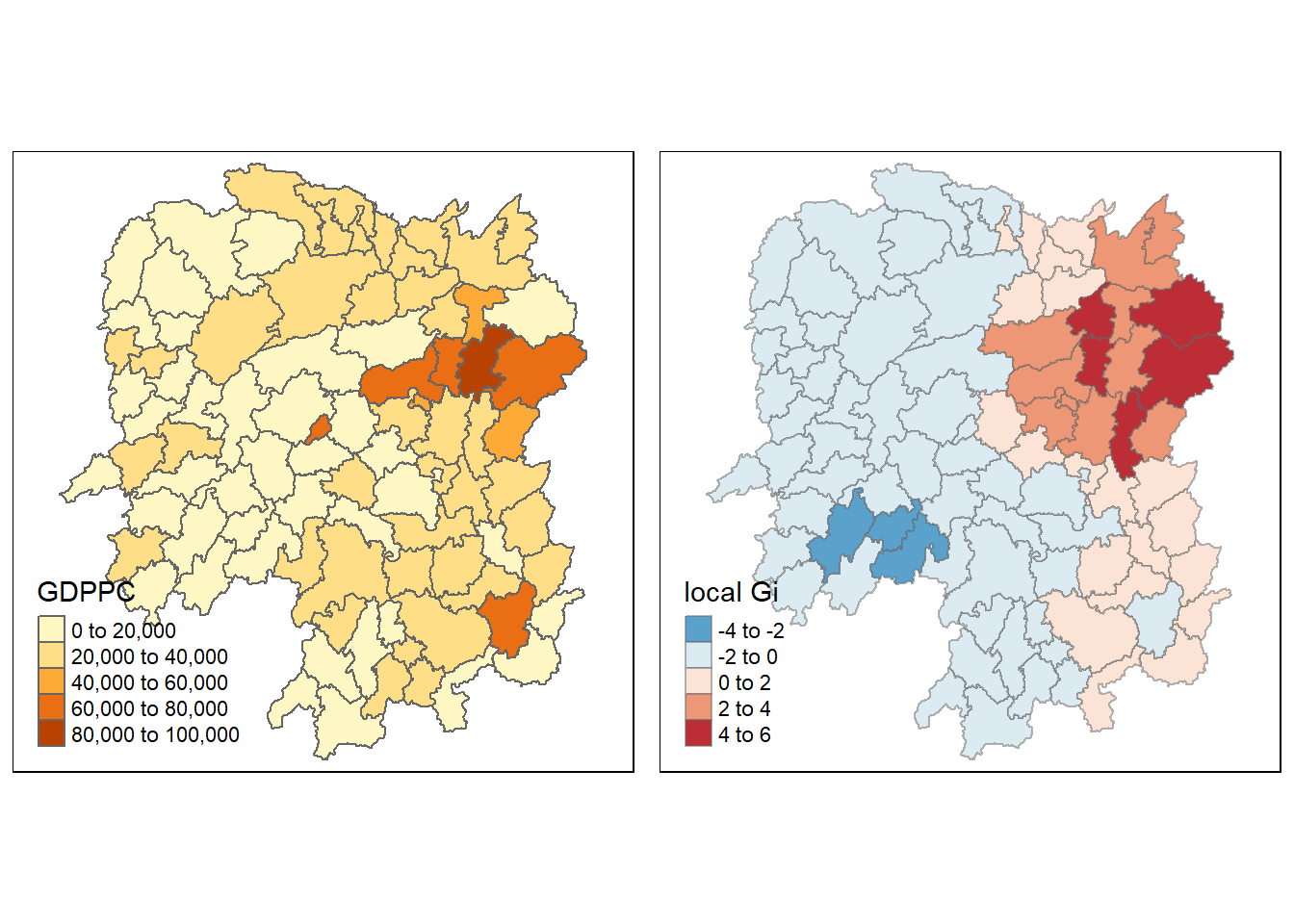
gdppc <- qtm(hunan, "GDPPC")

Gimap <-tm_shape(hunan.gi) +
  tm_fill(col = "gstat_fixed",
          style = "pretty",
          palette="-RdBu",
          title = "local Gi") +
  tm_borders(alpha = 0.5)

tmap_arrange(gdppc, Gimap, asp=1, ncol=2)
Variable(s) "gstat_fixed" contains positive and negative values, so midpoint is set to 0. Set midpoint = NA to show the full spectrum of the color palette.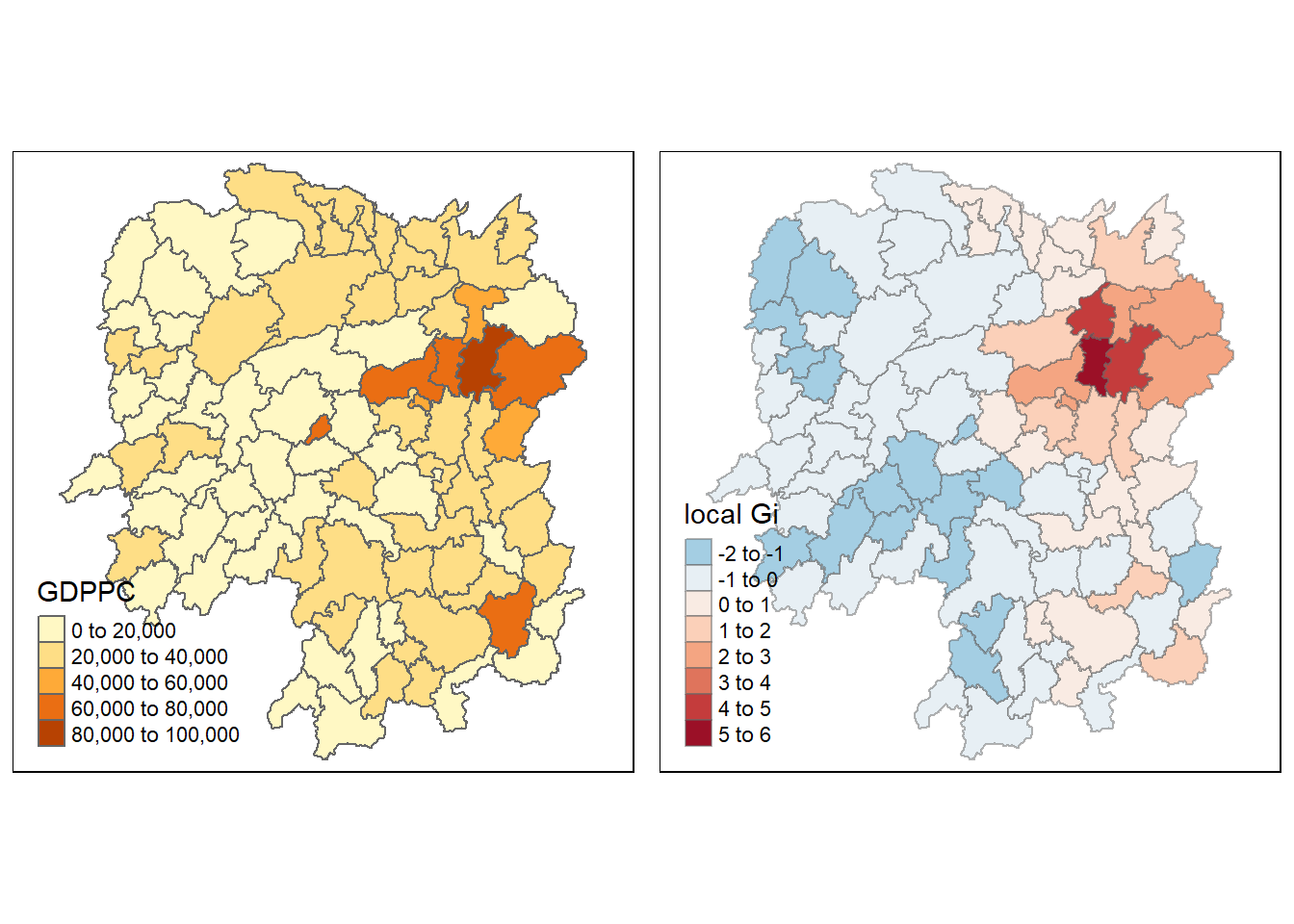
Gi statistics using adaptive distance
fips <- order(hunan$County)
gi.adaptive <- localG(hunan$GDPPC, knn_lw)
hunan.gi <- cbind(hunan, as.matrix(gi.adaptive)) %>%
  rename(gstat_adaptive = as.matrix.gi.adaptive.)
Mapping Gi values with adaptive distance weights
gdppc<- qtm(hunan, "GDPPC")

Gimap <- tm_shape(hunan.gi) +
  tm_fill(col = "gstat_adaptive",
          style = "pretty",
          palette="-RdBu",
          title = "local Gi") +
  tm_borders(alpha = 0.5)

tmap_arrange(gdppc,
             Gimap,
             asp=1,
             ncol=2)
Variable(s) "gstat_adaptive" contains positive and negative values, so midpoint is set to 0. Set midpoint = NA to show the full spectrum of the color palette.