pacman::p_load(maptools, sf, raster, spatstat, tmap,tidyverse,plotly,funModeling,sfdep)TakeHome_Ex1
Analysis on the geographic distribution of functional and non-function water points in Osub State, Nigeria
1.Background
Access to clean and abundant water is a vital necessity for human health and well-being. Adequate Clean water is crucial in promoting a healthy environment, sustaining economic growth in countries. However, a significant portion of the global population, including those in Nigeria, are still grappling with a lack of access to sufficient water resources. Given the critical role that water plays in many aspects of life, it is essential to understand the current water distribution system and identify potential areas for improvement.
2.Objectives
Apply appropriate spatial point patterns analysis method to discover the geographical distribution of functional and non-function water points an and their co-locations
3. Steps
3.1 Exploratory Spatial Data Analysis (ESDA)
3.1.1 Load necessary R-package and import the geospatial dataset
The package we used for analysis are:
sf: For importing, managing and processing vector-based geospatial data
tidyverse: For performing data science tasks such as importing, wrangling and visualising data.
tmap: used for creating thematic maps, such as choropleth and bubble maps
raster: reads, writes, manipulates, analyses and models gridded spatial data
spatstat: used for point pattern analysis
maptools: a set of tools for manipulating geographic data
funModeling: used for exploratory data analysis
sfdep: for performing geospatia data wrangling and local colocation quotient analysis.
Let’s load the package required!
Here are two possible datasets that we can obtain the geospatial information of Nigeria from, one is from Humanitarian Data Exchange portal, the other is from geoBoundaries, let’s read both of the datasets and examine which one is more suitable to use, notice that the crs for Nigeria should be 23692, so we need to assign the crs after reading the data:
geoNGA <- st_read("data/geospatial/",
layer = "geoBoundaries-NGA-ADM2") %>%
st_transform(crs = 26392)Reading layer `geoBoundaries-NGA-ADM2' from data source
`C:\Quanfang777\IS415-GAA\Takehome_Exercise\Takehome_Exercise1\data\geospatial'
using driver `ESRI Shapefile'
Simple feature collection with 774 features and 6 fields
Geometry type: MULTIPOLYGON
Dimension: XY
Bounding box: xmin: 2.668534 ymin: 4.273007 xmax: 14.67882 ymax: 13.89442
Geodetic CRS: WGS 84NGA <- st_read("data/geospatial/",
layer = "nga_admbnda_adm2_osgof_20190417") %>%
st_transform(crs = 26392)Reading layer `nga_admbnda_adm2_osgof_20190417' from data source
`C:\Quanfang777\IS415-GAA\Takehome_Exercise\Takehome_Exercise1\data\geospatial'
using driver `ESRI Shapefile'
Simple feature collection with 774 features and 16 fields
Geometry type: MULTIPOLYGON
Dimension: XY
Bounding box: xmin: 2.668534 ymin: 4.273007 xmax: 14.67882 ymax: 13.89442
Geodetic CRS: WGS 84After checking both sf dataframes, we notice that NGA provide both LGA and state information. Hence, NGA data.frame will be selected for the subsequent processing.
3.1.2 Importing Aspatial data
As our target is to analysis the water points in Osun State,Nigeria,(the area colored in red) so let’s filter the data and selected only the observations in Osun State, Nigeria
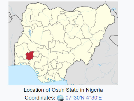
(Fig1: Location of Osun State)
wp_Osun <- read_csv("data/aspatial/WPdx.csv") %>%
filter(`#clean_country_name` == "Nigeria") %>%
filter (`#clean_adm1` == "Osun") Warning: One or more parsing issues, call `problems()` on your data frame for details,
e.g.:
dat <- vroom(...)
problems(dat)Rows: 406566 Columns: 70
── Column specification ────────────────────────────────────────────────────────
Delimiter: ","
chr (43): #source, #report_date, #status_id, #water_source_clean, #water_sou...
dbl (23): row_id, #lat_deg, #lon_deg, #install_year, #fecal_coliform_value, ...
lgl (4): #rehab_year, #rehabilitator, is_urban, latest_record
ℹ Use `spec()` to retrieve the full column specification for this data.
ℹ Specify the column types or set `show_col_types = FALSE` to quiet this message.3.1.3 Mapping the geospatial data sets
#Let's display the studyarea - Osun on the map:
NGA_Osun <- NGA%>%
filter(`ADM1_EN` == "Osun")Then, let’s ensure that spatial data to be used for analysis has no invalid geometries.
length(which(st_is_valid(NGA_Osun) == FALSE))[1] 0Plot the basemap for osun, Nigeria to check if we obtain the value correctly
osungraph = tmap_mode('plot')tmap mode set to plottingtm_shape(NGA_Osun)+tm_polygons()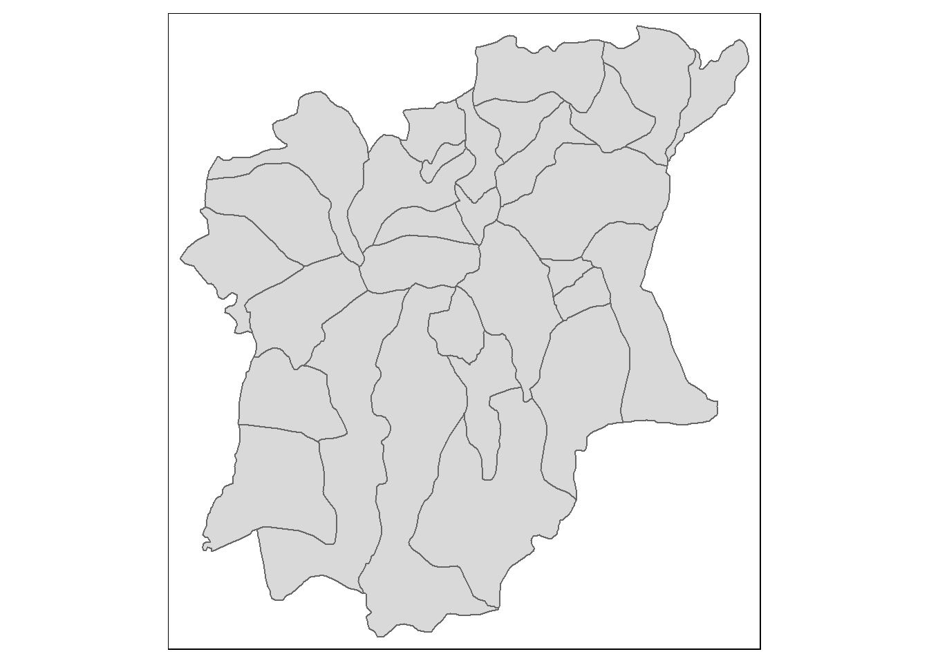
Compared to the map (Fig.1) we know that we have successfully obtained the geospatial information of Osun
3.1.4 Converting water point data into sf point features
In order to convert the point data into sf point feature for further analysis, first we need to convert the wkt field into sfc field by using st_as_sfc() data type.
wp_Osun$Geometry = st_as_sfc(wp_Osun$`New Georeferenced Column`)
wp_Osun# A tibble: 5,557 × 71
row_id `#source` #lat_…¹ #lon_…² #repo…³ #stat…⁴ #wate…⁵ #wate…⁶ #wate…⁷
<dbl> <chr> <dbl> <dbl> <chr> <chr> <chr> <chr> <chr>
1 429123 GRID3 8.02 5.06 08/29/… Unknown <NA> <NA> Tapsta…
2 70566 Federal Minis… 7.32 4.79 05/11/… No Protec… Well Mechan…
3 70578 Federal Minis… 7.76 4.56 05/11/… No Boreho… Well Mechan…
4 66401 Federal Minis… 8.03 4.64 04/30/… No Boreho… Well Mechan…
5 422190 GRID3 7.87 4.88 08/29/… Unknown <NA> <NA> Tapsta…
6 422064 GRID3 7.7 4.89 08/29/… Unknown <NA> <NA> Tapsta…
7 65607 Federal Minis… 7.89 4.71 05/12/… No Boreho… Well Mechan…
8 68989 Federal Minis… 7.51 4.27 05/07/… No Boreho… Well <NA>
9 67708 Federal Minis… 7.48 4.35 04/29/… Yes Boreho… Well Mechan…
10 66419 Federal Minis… 7.63 4.50 05/08/… Yes Boreho… Well Hand P…
# … with 5,547 more rows, 62 more variables: `#water_tech_category` <chr>,
# `#facility_type` <chr>, `#clean_country_name` <chr>, `#clean_adm1` <chr>,
# `#clean_adm2` <chr>, `#clean_adm3` <chr>, `#clean_adm4` <chr>,
# `#install_year` <dbl>, `#installer` <chr>, `#rehab_year` <lgl>,
# `#rehabilitator` <lgl>, `#management_clean` <chr>, `#status_clean` <chr>,
# `#pay` <chr>, `#fecal_coliform_presence` <chr>,
# `#fecal_coliform_value` <dbl>, `#subjective_quality` <chr>, …Then, use st_sf() to convert the tibble data.frame into sf object and also include the referencing system of the data into the sf object. ( Important, don’t forget to assign a crs when using st_sf)
wp_Osun <- st_sf(wp_Osun, crs=4326)
wp_OsunSimple feature collection with 5557 features and 70 fields
Geometry type: POINT
Dimension: XY
Bounding box: xmin: 4.032004 ymin: 7.060309 xmax: 5.06 ymax: 8.061898
Geodetic CRS: WGS 84
# A tibble: 5,557 × 71
row_id `#source` #lat_…¹ #lon_…² #repo…³ #stat…⁴ #wate…⁵ #wate…⁶ #wate…⁷
* <dbl> <chr> <dbl> <dbl> <chr> <chr> <chr> <chr> <chr>
1 429123 GRID3 8.02 5.06 08/29/… Unknown <NA> <NA> Tapsta…
2 70566 Federal Minis… 7.32 4.79 05/11/… No Protec… Well Mechan…
3 70578 Federal Minis… 7.76 4.56 05/11/… No Boreho… Well Mechan…
4 66401 Federal Minis… 8.03 4.64 04/30/… No Boreho… Well Mechan…
5 422190 GRID3 7.87 4.88 08/29/… Unknown <NA> <NA> Tapsta…
6 422064 GRID3 7.7 4.89 08/29/… Unknown <NA> <NA> Tapsta…
7 65607 Federal Minis… 7.89 4.71 05/12/… No Boreho… Well Mechan…
8 68989 Federal Minis… 7.51 4.27 05/07/… No Boreho… Well <NA>
9 67708 Federal Minis… 7.48 4.35 04/29/… Yes Boreho… Well Mechan…
10 66419 Federal Minis… 7.63 4.50 05/08/… Yes Boreho… Well Hand P…
# … with 5,547 more rows, 62 more variables: `#water_tech_category` <chr>,
# `#facility_type` <chr>, `#clean_country_name` <chr>, `#clean_adm1` <chr>,
# `#clean_adm2` <chr>, `#clean_adm3` <chr>, `#clean_adm4` <chr>,
# `#install_year` <dbl>, `#installer` <chr>, `#rehab_year` <lgl>,
# `#rehabilitator` <lgl>, `#management_clean` <chr>, `#status_clean` <chr>,
# `#pay` <chr>, `#fecal_coliform_presence` <chr>,
# `#fecal_coliform_value` <dbl>, `#subjective_quality` <chr>, …After assigning a crs to our sf object of wp_Osun, let’s transforming it into Nigeria projected coordinate system
wp_Osun <- wp_Osun %>%
st_transform(crs = 26392)Let’s if the crs has been assigned properly!
st_crs(wp_Osun)Coordinate Reference System:
User input: EPSG:26392
wkt:
PROJCRS["Minna / Nigeria Mid Belt",
BASEGEOGCRS["Minna",
DATUM["Minna",
ELLIPSOID["Clarke 1880 (RGS)",6378249.145,293.465,
LENGTHUNIT["metre",1]]],
PRIMEM["Greenwich",0,
ANGLEUNIT["degree",0.0174532925199433]],
ID["EPSG",4263]],
CONVERSION["Nigeria Mid Belt",
METHOD["Transverse Mercator",
ID["EPSG",9807]],
PARAMETER["Latitude of natural origin",4,
ANGLEUNIT["degree",0.0174532925199433],
ID["EPSG",8801]],
PARAMETER["Longitude of natural origin",8.5,
ANGLEUNIT["degree",0.0174532925199433],
ID["EPSG",8802]],
PARAMETER["Scale factor at natural origin",0.99975,
SCALEUNIT["unity",1],
ID["EPSG",8805]],
PARAMETER["False easting",670553.98,
LENGTHUNIT["metre",1],
ID["EPSG",8806]],
PARAMETER["False northing",0,
LENGTHUNIT["metre",1],
ID["EPSG",8807]]],
CS[Cartesian,2],
AXIS["(E)",east,
ORDER[1],
LENGTHUNIT["metre",1]],
AXIS["(N)",north,
ORDER[2],
LENGTHUNIT["metre",1]],
USAGE[
SCOPE["Engineering survey, topographic mapping."],
AREA["Nigeria between 6°30'E and 10°30'E, onshore and offshore shelf."],
BBOX[3.57,6.5,13.53,10.51]],
ID["EPSG",26392]]3.1.5 Geospatial Data Cleaning
Checking for duplicate name
It is always important for us to check for duplicate name in the data main data fields. Here are the steps of properly handling the duplication
# Get all the duplicated LGA names
duplicated_LGA <- NGA_Osun$ADM2_EN[duplicated(NGA_Osun$ADM2_EN)==TRUE]
# Get all the indices with names that are included in the duplicated LGA names
duplicated_indices <- which(NGA_Osun$ADM2_EN %in% duplicated_LGA)
# For every index in the duplicated_indices, concatenate the two columns with a comma
for (ind in duplicated_indices) {
NGA_Osun$ADM2_EN[ind] <- paste(NGA_Osun$ADM2_EN[ind], NGA_Osun$ADM1_EN[ind], sep=", ")
}Let’s confirm if there is any duplication
NGA_Osun$ADM2_EN[duplicated(NGA_Osun$ADM2_EN)==TRUE]character(0)Great, let’s moving on
3.1.6 Data Wrangling for Water Point Data
Let’s have a quick understanding of our water point data
freq(data = wp_Osun,
input = '#status_clean')Warning: The `<scale>` argument of `guides()` cannot be `FALSE`. Use "none" instead as
of ggplot2 3.3.4.
ℹ The deprecated feature was likely used in the funModeling package.
Please report the issue at <https://github.com/pablo14/funModeling/issues>.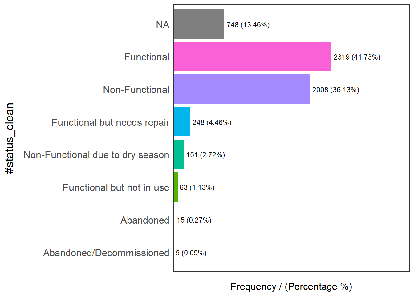
#status_clean frequency percentage cumulative_perc
1 Functional 2319 41.73 41.73
2 Non-Functional 2008 36.13 77.86
3 <NA> 748 13.46 91.32
4 Functional but needs repair 248 4.46 95.78
5 Non-Functional due to dry season 151 2.72 98.50
6 Functional but not in use 63 1.13 99.63
7 Abandoned 15 0.27 99.90
8 Abandoned/Decommissioned 5 0.09 100.00We can see that there are 9 classes in the #status_clean field, and there is a class called NA, for easy handling the subsequent steps and make it a more meaningful analysis, we can do following:
Recode the NA values into unknown
Remove the ‘#’ sign before the #status_clean field
9 classes are a lot, and it is possible to combine them into 3 meaningful classes
#recode the NA values into unknown and remove the '#'sign before #status_clean field
wp_Osun <- wp_Osun %>%
rename(status_clean = '#status_clean') %>%
select(status_clean) %>%
mutate(status_clean = replace_na(
status_clean, "unknown"))3.1.7 Extracting Water Point Data and combine them into 3 meaningful classes
Now, let’s extract the water point data in Osun state according to their status.
To extract functional water point:
wp_Osun_functional <- wp_Osun %>%
filter(status_clean %in%
c("Functional",
"Functional but not in use",
"Functional but needs repair"))To extract non-functional water point:
wp_Osun_nonfunctional <- wp_Osun %>%
filter(status_clean %in%
c("Abandoned/Decommissioned",
"Abandoned",
"Non-Functional due to dry season",
"Non-Functional",
"Non functional due to dry season"))To extract water point with unknown status
wp_Osun_unknown <- wp_Osun %>%
filter(status_clean == "unknown")3.2 Display the kernel density maps on openstreetmap of Osub State, Nigeria.
For displaying the kernel density maps, many geospatial analysis packages required need the input geospatial data to be in sp’s Spatial* classes, so we need to convert simple feature data frame to sp’s Spatial* class.
3.2.1 convert simple feature data frame to sp’s Spatial* class.
wp_Osun_functional <- as_Spatial(wp_Osun_functional)
wp_Osun_nonfunctional<- as_Spatial(wp_Osun_nonfunctional)
NGA_Osun_sp <- as_Spatial(NGA_Osun)3.2.2 Converting the Spatial* class into generic sp format
For further analysis, we need spatstat which requires the analytical data in ppp object form. There is no direct way to convert a Spatial* classes into ppp object. We need to convert the Spatial classes* into Spatial object first.
Spatial classes-> Spatial object (Spatial classes usually contains more information than Spatial object, Spatial object only contains the spatial information so it has lesser time to process)
wp_Osun_functional_sp <- as(wp_Osun_functional, "SpatialPoints")
wp_Osun_nonfunctional_sp <- as(wp_Osun_nonfunctional, "SpatialPoints")
NGA_Osun_sp<- as(NGA_Osun_sp, "SpatialPolygons")3.2.3 Converting the generic sp format into spatstat’s ppp format
Now, we will use as.ppp() function of spatstat to convert the spatial data into spatstat’s ppp object format, let’s do it for both functional and non-function waterpoint data
wp_Osun_functional_ppp <- as(wp_Osun_functional, "ppp")
wp_Osun_functional_pppMarked planar point pattern: 2630 points
marks are of storage type 'character'
window: rectangle = [177285.9, 290750.96] x [343128.1, 450859.7] unitswp_Osun_nonfunctional_ppp <- as(wp_Osun_nonfunctional, "ppp")
wp_Osun_nonfunctional_pppMarked planar point pattern: 2179 points
marks are of storage type 'character'
window: rectangle = [180538.96, 290616] x [340054.1, 450780.1] units3.2.4 Handling duplicated points
It is always important to check if there are duplicated points!
any(duplicated(wp_Osun_functional_ppp))[1] FALSEany(duplicated(wp_Osun_nonfunctional_ppp))[1] FALSEThere is no duplication point, let’s moving on!
3.2.5 Creating owin object
When analysing spatial point patterns, it will be good to confine the analysis with a geographical area, in this case, let’s confine the analysis within Osun boundary. In spatstat, an object called owin is specially designed to represent this polygonal region.
Osun_owin <- as(NGA_Osun_sp, "owin")plot(Osun_owin)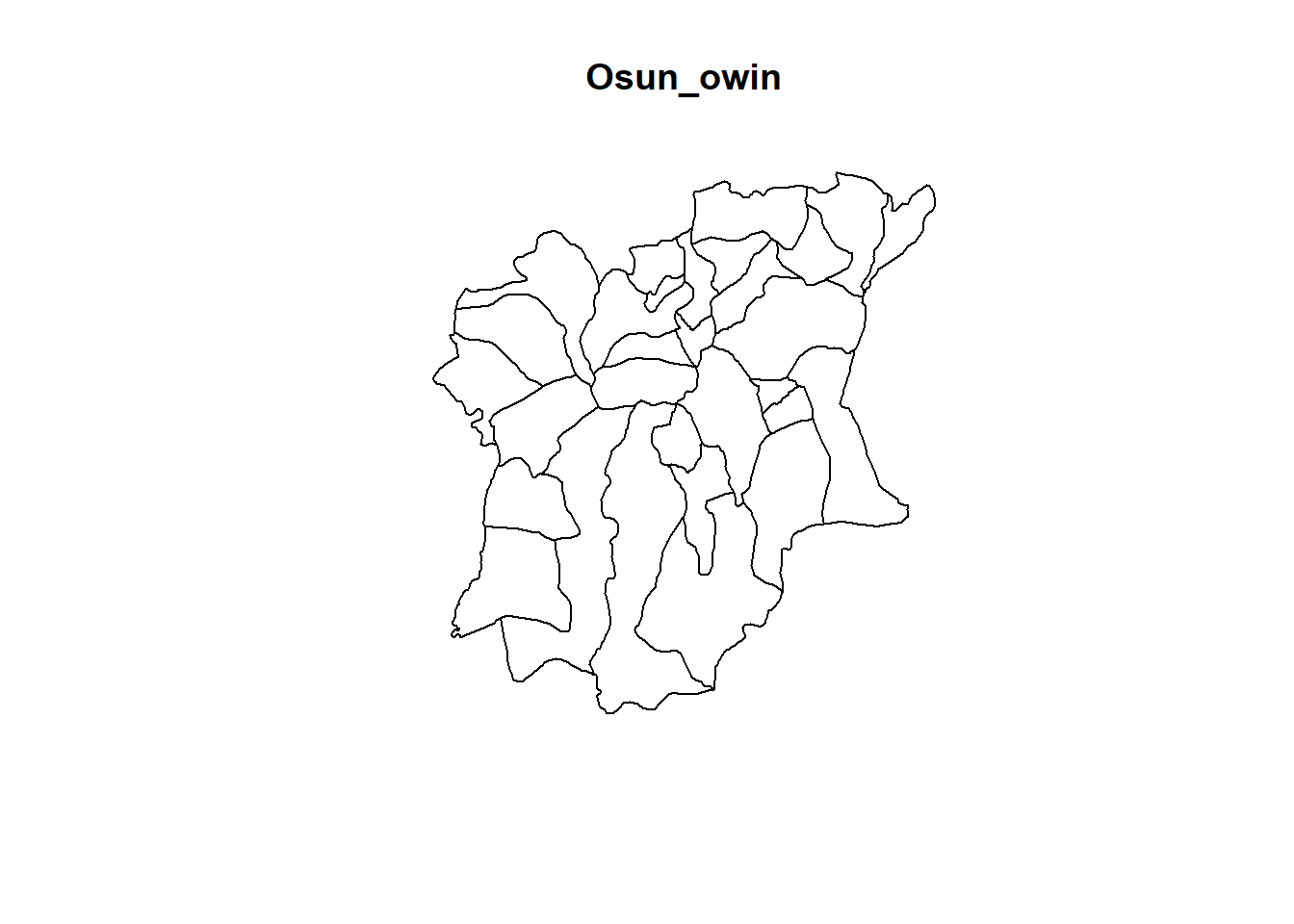
3.2.6 Combining point events object and owin object
Now, let’s combine both the point and polygon feature in ppp object class
wp_Osun_functional_ppp = wp_Osun_functional_ppp[Osun_owin]
wp_Osun_nonfunctional_ppp = wp_Osun_nonfunctional_ppp[Osun_owin]3.2.7 Start First-order Spatial Point Patterns Analysis
Let’s compute the Kernel Density map for both functional waterpoint and nonfunctional waterpoint in Osun
Let’s use bw.diggle() to compute an ideal bandwidth selection method for us and use “gaussian” for our smoothing method
kde_Osun_functional_bw<- density(wp_Osun_functional_ppp,
sigma=bw.diggle,
edge=TRUE,
kernel="gaussian") kde_Osun_nonfunctional_bw<- density(wp_Osun_nonfunctional_ppp,
sigma=bw.diggle,
edge=TRUE,
kernel="gaussian") plot(kde_Osun_functional_bw)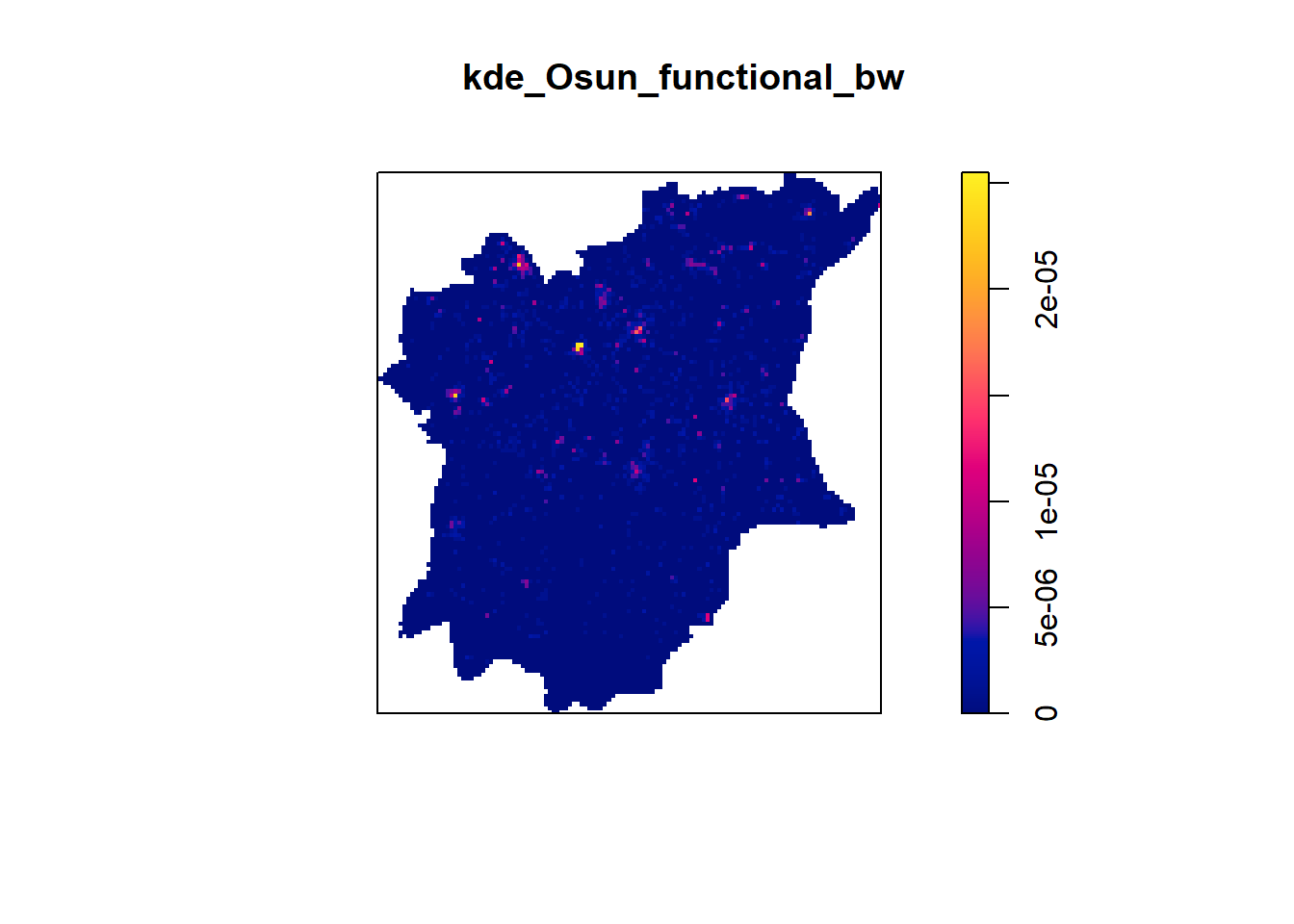
The density values of the output range from 0 to 0.00002 which is way too small to comprehend. This is because the default unit of measurement is in meter. As a result, the density values computed is in “number of points per square meter”. so, let’s rescale our KDE values
3.2.8 Rescaling KDE values
Let’s convert the unit of measurement from meter to kilometer.
wp_Osun_functional_ppp.km <- rescale(wp_Osun_functional_ppp, 1000, "km")wp_Osun_nonfunctional_ppp.km <- rescale(wp_Osun_nonfunctional_ppp, 1000, "km")Now, let’s plot the map after rescaling
kde_Osun_functional.bw <- density(wp_Osun_functional_ppp.km, sigma=bw.diggle, edge=TRUE, kernel="gaussian")
plot(kde_Osun_functional.bw)
kde_Osun_nonfunctional.bw <- density(wp_Osun_nonfunctional_ppp.km, sigma=bw.diggle, edge=TRUE, kernel="gaussian")
plot(kde_Osun_nonfunctional.bw)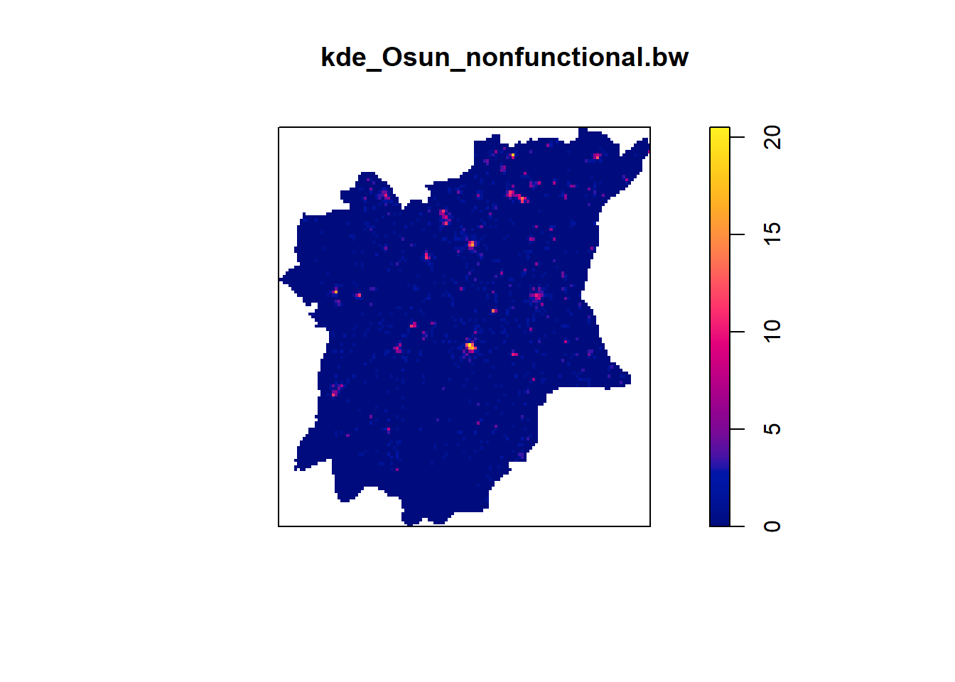
Fixed bandwidth method is very sensitive to highly skew distribution of spatial point patterns over geographical units for example urban versus rural. One way to overcome this problem is by using adaptive bandwidth instead.
This is the code to compute adaptive bandwidth
wp_Osun_functional_adaptive <- adaptive.density(wp_Osun_functional_ppp.km, method="kernel")
plot(wp_Osun_functional_adaptive)
wp_Osun_nonfunctional_adaptive <- adaptive.density(wp_Osun_nonfunctional_ppp.km, method="kernel")
plot(wp_Osun_nonfunctional_adaptive)
We can compare the fixed and adaptive kernel density estimation outputs by using the code chunk below.
3.2.9 Function waterpoint distribution in fixed and adaptive kernel density estimation outputs
par(mfrow=c(1,2))
plot(kde_Osun_functional.bw, main = "Fixed bandwidth")
plot(wp_Osun_functional_adaptive, main = "Adaptive bandwidth")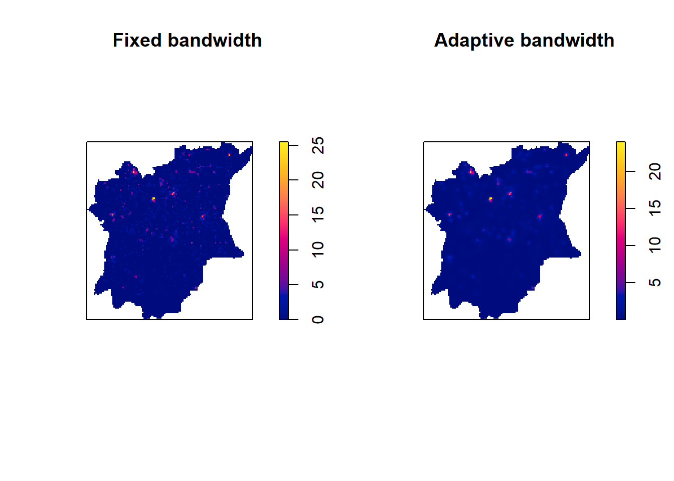
Nonfunctional waterpoint distribution in fixed and adaptive kernel density estimation outputs
par(mfrow=c(1,2))
plot(kde_Osun_nonfunctional.bw, main = "Fixed bandwidth")
plot(wp_Osun_nonfunctional_adaptive, main = "Adaptive bandwidth")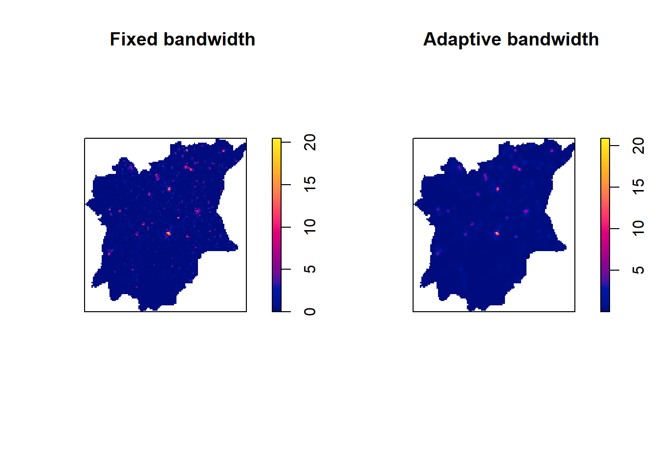
3.2.10 Converting KDE output into grid object.
We need to convert the KDE output so that it is suitable for mapping purposes
kde_functionalwp_raster <- kde_Osun_functional.bw %>%
as.SpatialGridDataFrame.im() %>%
raster()
kde_functionalwp_rasterclass : RasterLayer
dimensions : 128, 128, 16384 (nrow, ncol, ncell)
resolution : 0.8948485, 0.9616045 (x, y)
extent : 176.5032, 291.0438, 331.4347, 454.5201 (xmin, xmax, ymin, ymax)
crs : NA
source : memory
names : v
values : -5.092436e-15, 25.49435 (min, max)kde_nonfunctionalwp_raster <- kde_Osun_nonfunctional.bw %>%
as.SpatialGridDataFrame.im() %>%
raster()
kde_nonfunctionalwp_rasterclass : RasterLayer
dimensions : 128, 128, 16384 (nrow, ncol, ncell)
resolution : 0.8948485, 0.9616045 (x, y)
extent : 176.5032, 291.0438, 331.4347, 454.5201 (xmin, xmax, ymin, ymax)
crs : NA
source : memory
names : v
values : -3.925434e-15, 20.49412 (min, max)3.2.11 Assign projection
projection(kde_functionalwp_raster) <- CRS('+init=EPSG:26392')
projection(kde_nonfunctionalwp_raster) <- CRS('+init=EPSG:26392')
kde_functionalwp_rasterclass : RasterLayer
dimensions : 128, 128, 16384 (nrow, ncol, ncell)
resolution : 0.8948485, 0.9616045 (x, y)
extent : 176.5032, 291.0438, 331.4347, 454.5201 (xmin, xmax, ymin, ymax)
crs : +proj=tmerc +lat_0=4 +lon_0=8.5 +k=0.99975 +x_0=670553.98 +y_0=0 +a=6378249.145 +rf=293.465 +units=m +no_defs
source : memory
names : v
values : -5.092436e-15, 25.49435 (min, max)kde_nonfunctionalwp_rasterclass : RasterLayer
dimensions : 128, 128, 16384 (nrow, ncol, ncell)
resolution : 0.8948485, 0.9616045 (x, y)
extent : 176.5032, 291.0438, 331.4347, 454.5201 (xmin, xmax, ymin, ymax)
crs : +proj=tmerc +lat_0=4 +lon_0=8.5 +k=0.99975 +x_0=670553.98 +y_0=0 +a=6378249.145 +rf=293.465 +units=m +no_defs
source : memory
names : v
values : -3.925434e-15, 20.49412 (min, max)3.2.12 Visualizing the output in tmap Openstreet and describe the spatial patterns
The functional water point distribution
tmap_mode('view')tmap mode set to interactive viewingtm_basemap('OpenStreetMap') +
tm_shape(kde_functionalwp_raster) +
tm_raster('v') +
tm_layout(legend.position = c('right', 'bottom'),
frame = FALSE)legend.postion is used for plot mode. Use view.legend.position in tm_view to set the legend position in view mode.Variable(s) "v" contains positive and negative values, so midpoint is set to 0. Set midpoint = NA to show the full spectrum of the color palette.The nonfunctional water point distribution
tmap_mode('view')tmap mode set to interactive viewingtm_basemap('OpenStreetMap') +
tm_shape(kde_nonfunctionalwp_raster) +
tm_raster('v') +
tm_layout(legend.position = c('right', 'bottom'),
frame = FALSE)legend.postion is used for plot mode. Use view.legend.position in tm_view to set the legend position in view mode.Variable(s) "v" contains positive and negative values, so midpoint is set to 0. Set midpoint = NA to show the full spectrum of the color palette.From the graph we can clearly see that the nonfunctional waterpoints are centered in the central region area (IFE Central). When compare these two maps above (functional waterpoint distribution and non functional waterpoint distribution), we found the north part of Osun has more functional waterpoints than the south part of Osun
3.1.13 Plot Point Map
tmap_mode("view")tmap mode set to interactive viewingtm_shape(NGA_Osun) +
tm_polygons() +
tm_shape(wp_Osun)+
tm_dots(col = "status_clean",
size = 0.01,
border.col = "black",
border.lwd = 0.5) +
tm_view(set.zoom.limits = c(8, 16))It looks like the graph has too many colors and it will be better if we group them only in Functional, Nonfunctional, Unknown, so it will be clear to visualize
wp_Osun <- wp_Osun %>%
mutate(status_group = recode(status_clean,
"Functional" = "Functional",
"Functional but not in use" = "Functional",
"Functional but needs repair" = "Functional",
"Abandoned/Decommissioned" = "Nonfunctional",
"Abandoned" = "Nonfunctional",
"Non-Functional due to dry season" = "Nonfunctional",
"Non-Functional" = "Nonfunctional",
"Non functional due to dry season" = "Nonfunctional",
"unknown" = "Unknown"))tmap_mode("view")tmap mode set to interactive viewingtm_shape(NGA_Osun) +
tm_polygons() +
tm_shape(wp_Osun)+
tm_dots(col = "status_group",
size = 0.01,
border.col = "black",
border.lwd = 0.5) +
tm_view(set.zoom.limits = c(8, 16))plot(kde_Osun_functional.bw, main = "Functional Waterpoint")
plot(kde_Osun_nonfunctional.bw, main = "Nonfunctional Waterpoint")
The advantage of kernel density map over point map:
Kernel density map can provide us with a clear representation of the spatial data distribution. It provides a smooth representation of the underlying distribution and make sure the visualization of areas with a high concentration of points is clear, while point maps can be misleading because they may over-represent areas with many points and under-represent areas with fewer points. In our case, we can see when there are so many points on the graph of point map, it is very hard to observe and interpret.
3.3 Second-order Spatial Point Patterns Analysis
L function is a tool used to analyze spatial point patterns. It is a summary statistic that provides information on the spatial distribution of points.The L function can be used to identify clustering or regularity in the distribution of points, as well as to assess the spatial randomness of the point pattern.
Here is the code to
3.3.1 perform L function
#to run this code, remove the'#'
#L_ck = Lest(wp_Osun_functional_ppp, correction = "Ripley")
#plot(L_ck, . -r ~ r,
#ylab= "L(d)-r", xlab = "d(m)")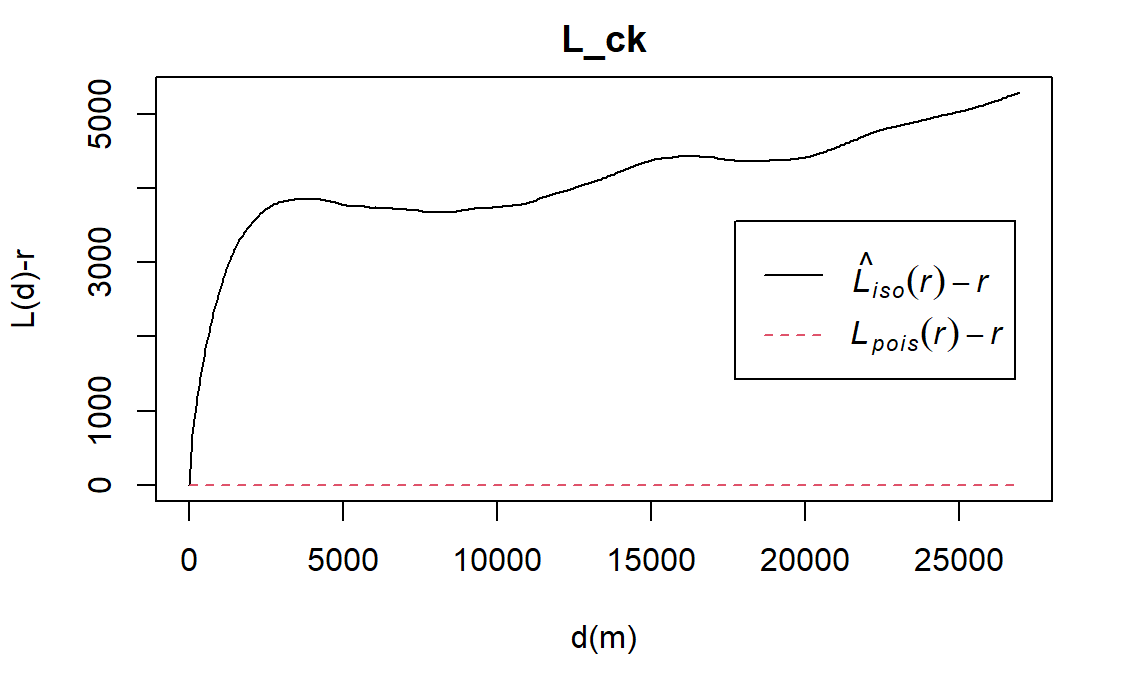
#L_ck = Lest(wp_Osun_nonfunctional_ppp, correction = "Ripley")
#plot(L_ck, . -r ~ r,
#ylab= "L(d)-r", xlab = "d(m)")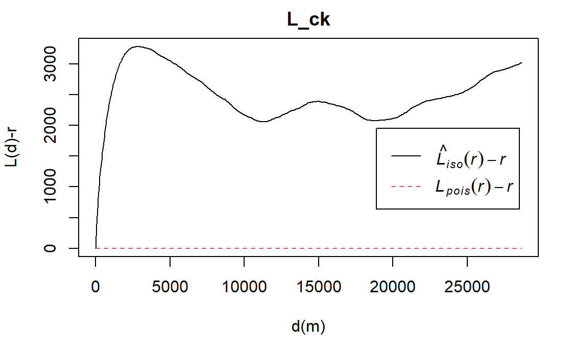
3.3.2 Performing Complete Spatial Randomness Test
To confirm the observed spatial patterns above, a hypothesis test will be conducted. The hypothesis and test are as follows:
Ho = The distribution of the functional/nonfunctional water point in Osun are randomly distributed.
H1= The distribution of the functional/nonfunctional water point in Osun are not randomly distributed.
The null hypothesis will be rejected if p-value if smaller than alpha value of 0.001.
The code chunk below is used to perform the hypothesis testing.
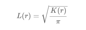
The L function is a variance-stabilising transformation of the K function:
Methodology and Interpretation
To assess the spatial point pattern, (L(r)−r) will be plotted against r
At complete spatial randomness (CSR), L(r)−r=0
L(r)–r>0 implies clustering
L(r)−r<0 implies dispersion
#L_ck.csr <- envelope(wp_Osun_functional_ppp, Lest, nsim = 5, rank = 1, glocal=TRUE)#plot(L_ck.csr, . - r ~ r, xlab="d", ylab="L(d)-r")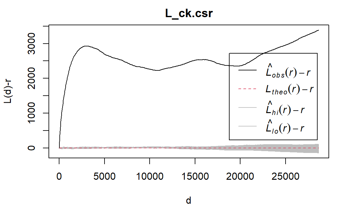
#L_ck.csr <- envelope(wp_Osun_nonfunctional_ppp, Lest, nsim = 5, rank = 1, glocal=TRUE)#plot(L_ck.csr, . - r ~ r, xlab="d", ylab="L(d)-r")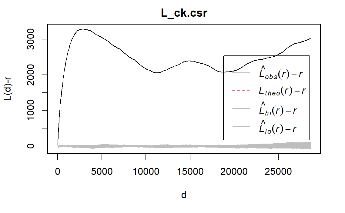
3.3.2 Given analysis results, draw statistical conclusions
The L(r)−r function for both functional and nonfunctional water points in Osun (black line) lies above the L(r)−r function at CSR (red line), suggesting clustering. Meanwhile, all of the observed L(r)−r values go above of the randomisation envelope, suggesting statistically significant clustering of both functional and nonfunctional waterpoints in Osun
3.4 Spatial Correlation Analysis
In the code chunk below, st_knn() of sfdep package is used to determine the k (i.e. 6) nearest neighbours for given point geometry.
nb <- include_self(
st_knn(st_geometry(wp_Osun), 6))st_kernel_weights() of sfdep package is used to derive a weights list by using a kernel function.
wt <- st_kernel_weights(nb,
wp_Osun,
"gaussian",
adaptive = TRUE)To compute LCLQ by using sfdep package, the reference point data must be in either character or vector list. The code chunks below are used to prepare two vector lists. One of FunctionalWaterpoint and NonFunctionalWaterpoint are called A and B respectively.
FunctionalWaterpoint <- wp_Osun %>%
filter(status_group == "Functional")
A<- FunctionalWaterpoint$status_groupNonFunctionalWaterpoint <- wp_Osun %>%
filter(status_group == "Nonfunctional")
B <- NonFunctionalWaterpoint$status_grouplocal_colocation() us used to compute the LCLQ values for each NonFunctional water point event.
LCLQ <- local_colocation(B, A, nb, wt, 49)Joining output table
LCLQ_waterpoint <- cbind(wp_Osun, LCLQ)tmap_mode("view")tmap mode set to interactive viewingtm_shape(NGA_Osun) +
tm_polygons() +
tm_shape(LCLQ_waterpoint)+
tm_dots(col = "p_sim_Functional",
size = 0.01,
border.col = "black",
border.lwd = 0.5) +
tm_view(set.zoom.limits = c(8, 16))From the graph, the water point with p-value is small (less than 0.05) is highlighted in color, for the above code, we use non-functional waterpoint as our Category of Interest, the point highlighted in yellow color means that the actual co-location quotient for those nonfunctional water points is statistically significant. Those non-functional water point are surrounded with functional water points and should be carefully examined