Handon_Ex06

Spatial Weights and Applications

Overview

Learning objective:

import geospatial data using appropriate function(s) of sf package,
import csv file using appropriate function of readr package,
perform relational join using appropriate join function of dplyr package,
compute spatial weights using appropriate functions of spdep package, and
calculate spatially lagged variables using appropriate functions of spdep package.

The Study Area and Data

Two data sets will be used in this hands-on exercise, they are:

Hunan county boundary layer. This is a geospatial data set in ESRI shapefile format.
Hunan_2012.csv: This csv file contains selected Hunan's local development indicators in 2012.

Getting Started

pacman::p_load(sf, spdep, tmap, tidyverse, knitr)

Getting the Data Into R Environment

hunan <- st_read(dsn = "data/geospatial", 
                 layer = "Hunan")

Reading layer `Hunan' from data source 
  `C:\Quanfang777\IS415-GAA\WeeklyExercise\week6\Hands-on_Ex06\data\geospatial' 
  using driver `ESRI Shapefile'
Simple feature collection with 88 features and 7 fields
Geometry type: POLYGON
Dimension:     XY
Bounding box:  xmin: 108.7831 ymin: 24.6342 xmax: 114.2544 ymax: 30.12812
Geodetic CRS:  WGS 84

hunan2012 <- read_csv("data/aspatial/Hunan_2012.csv")

Rows: 88 Columns: 29
── Column specification ────────────────────────────────────────────────────────
Delimiter: ","
chr  (2): County, City
dbl (27): avg_wage, deposite, FAI, Gov_Rev, Gov_Exp, GDP, GDPPC, GIO, Loan, ...

ℹ Use `spec()` to retrieve the full column specification for this data.
ℹ Specify the column types or set `show_col_types = FALSE` to quiet this message.

Performing relational join

hunan <- left_join(hunan,hunan2012)%>%
  select(1:4, 7, 15)  #why six column

Joining, by = "County"

Visualising Regional Development Indicator

basemap <- tm_shape(hunan) +
  tm_polygons() +
  tm_text("NAME_3", size=0.5)

gdppc <- qtm(hunan, "GDPPC")
tmap_arrange(basemap, gdppc, asp=1, ncol=2)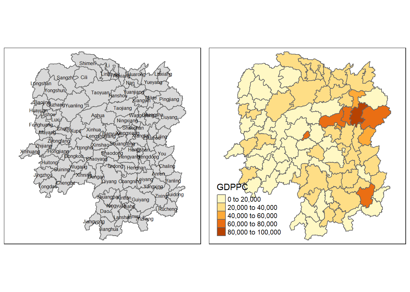

Computing Contiguity Spatial Weights

wm_q <- poly2nb(hunan, queen=TRUE)
summary(wm_q)

Neighbour list object:
Number of regions: 88 
Number of nonzero links: 448 
Percentage nonzero weights: 5.785124 
Average number of links: 5.090909 
Link number distribution:

 1  2  3  4  5  6  7  8  9 11 
 2  2 12 16 24 14 11  4  2  1 
2 least connected regions:
30 65 with 1 link
1 most connected region:
85 with 11 links

The summary report above shows that there are 88 area units in Hunan. The most connected area unit has 11 neighbours. There are two area units with only one heighbours.

For each polygon in our polygon object, wm_q lists all neighboring polygons. For example, to see the neighbors for the first polygon in the object, type:

wm_q[[1]]

[1]  2  3  4 57 85

#this showing the neighour of city id 1

hunan$County[1]

[1] "Anxiang"

To reveal the county names of the five neighboring polygons, the code chunk will be used:

hunan$NAME_3[c(2,3,4,57,85)]

[1] "Hanshou" "Jinshi"  "Li"      "Nan"     "Taoyuan"

nb1 <- wm_q[[1]]
nb1 <- hunan$GDPPC[nb1]
nb1

[1] 20981 34592 24473 21311 22879

The printed output above shows that the GDPPC of the five nearest neighbours based on Queen's method are 20981, 34592, 24473, 21311 and 22879 respectively.

Row-standardised weights matrix

Next, we need to assign weights to each neighboring polygon. In our case, each neighboring polygon will be assigned equal weight (style="W"). This is accomplished by assigning the fraction 1/(#ofneighbors) to each neighboring county then summing the weighted income values. While this is the most intuitive way to summaries the neighbors' values it has one drawback in that polygons along the edges of the study area will base their lagged values on fewer polygons thus potentially over- or under-estimating the true nature of the spatial autocorrelation in the data. For this example, we'll stick with the style="W" option for simplicity's sake but note that other more robust options are available, notably style="B".

rswm_q <- nb2listw(wm_q, 
                   style="W", 
                   zero.policy = TRUE)
rswm_q

Characteristics of weights list object:
Neighbour list object:
Number of regions: 88 
Number of nonzero links: 448 
Percentage nonzero weights: 5.785124 
Average number of links: 5.090909 

Weights style: W 
Weights constants summary:
   n   nn S0       S1       S2
W 88 7744 88 37.86334 365.9147

The input of nb2listw() must be an object of class nb. The syntax of the function has two major arguments, namely style and zero.poly.

style can take values “W”, “B”, “C”, “U”, “minmax” and “S”. B is the basic binary coding, W is row standardised (sums over all links to n), C is globally standardised (sums over all links to n), U is equal to C divided by the number of neighbours (sums over all links to unity), while S is the variance-stabilizing coding scheme proposed by Tiefelsdorf et al. 1999, p. 167-168 (sums over all links to n).

If zero policy is set to TRUE, weights vectors of zero length are inserted for regions without neighbour in the neighbours list. These will in turn generate lag values of zero, equivalent to the sum of products of the zero row t(rep(0, length=length(neighbours))) %*% x, for arbitrary numerical vector x of length length(neighbours). The spatially lagged value of x for the zero-neighbour region will then be zero, which may (or may not) be a sensible choice.

Global Spatial Autocorrelation: Moran's

Maron's I test

The code chunk below performs Moran’s I statistical testing using moran.test() of spdep.

moran.test(hunan$GDPPC, 
           listw=rswm_q, 
           zero.policy = TRUE, 
           na.action=na.omit)


    Moran I test under randomisation

data:  hunan$GDPPC  
weights: rswm_q    

Moran I statistic standard deviate = 4.7351, p-value = 1.095e-06
alternative hypothesis: greater
sample estimates:
Moran I statistic       Expectation          Variance 
      0.300749970      -0.011494253       0.004348351

The code chunk below performs permutation test for Moran's I statistic by using moran.mc() of spdep. A total of 1000 simulation will be performed

set.seed(1234)
bperm= moran.mc(hunan$GDPPC, 
                listw=rswm_q, 
                nsim=999, 
                zero.policy = TRUE, 
                na.action=na.omit)
bperm


    Monte-Carlo simulation of Moran I

data:  hunan$GDPPC 
weights: rswm_q  
number of simulations + 1: 1000 

statistic = 0.30075, observed rank = 1000, p-value = 0.001
alternative hypothesis: greater

Visualising Monte Carlo Moran's I

hist(bperm$res, 
     freq=TRUE, 
     breaks=20, 
     xlab="Simulated Moran's I")
abline(v=0, 
       col="red")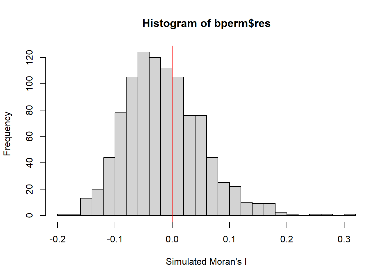

Global Spatial Autocorrelation: Geary's

geary.test(hunan$GDPPC, listw=rswm_q)


    Geary C test under randomisation

data:  hunan$GDPPC 
weights: rswm_q 

Geary C statistic standard deviate = 3.6108, p-value = 0.0001526
alternative hypothesis: Expectation greater than statistic
sample estimates:
Geary C statistic       Expectation          Variance 
        0.6907223         1.0000000         0.0073364

Computing Monte Carlo Geary's C

set.seed(1234)
bperm=geary.mc(hunan$GDPPC, 
               listw=rswm_q, 
               nsim=999)
bperm


    Monte-Carlo simulation of Geary C

data:  hunan$GDPPC 
weights: rswm_q 
number of simulations + 1: 1000 

statistic = 0.69072, observed rank = 1, p-value = 0.001
alternative hypothesis: greater

hist(bperm$res, freq=TRUE, breaks=20, xlab="Simulated Geary c")
abline(v=1, col="red")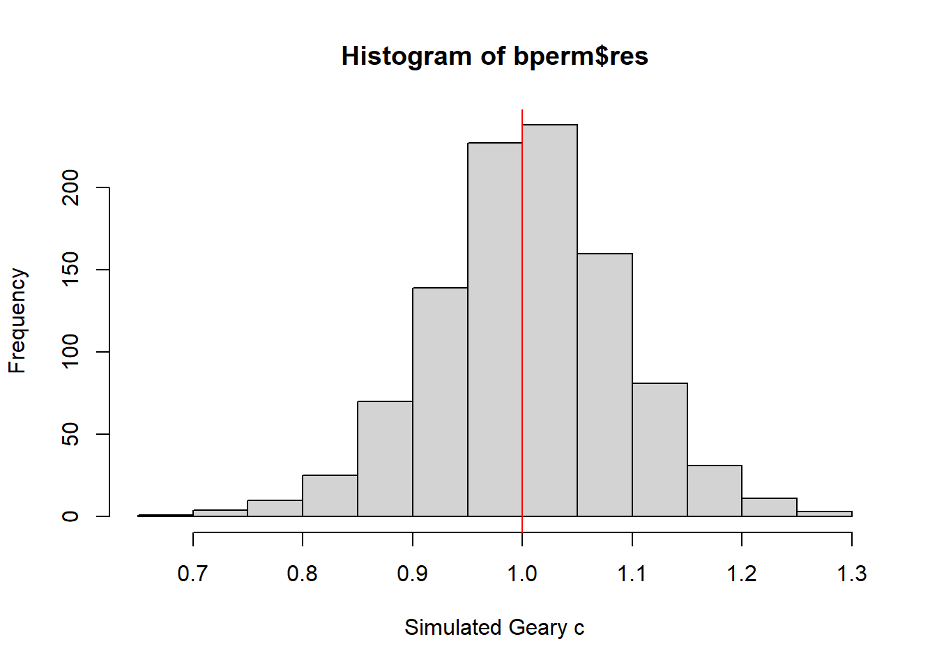

Compute Moran's I correlogram

MI_corr <- sp.correlogram(wm_q, 
                          hunan$GDPPC, 
                          order=6, 
                          method="I", 
                          style="W")
plot(MI_corr)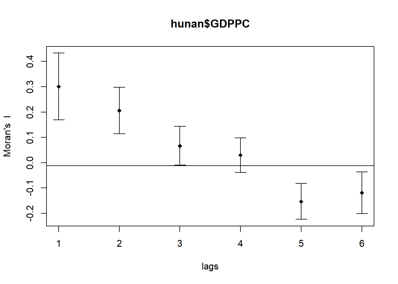

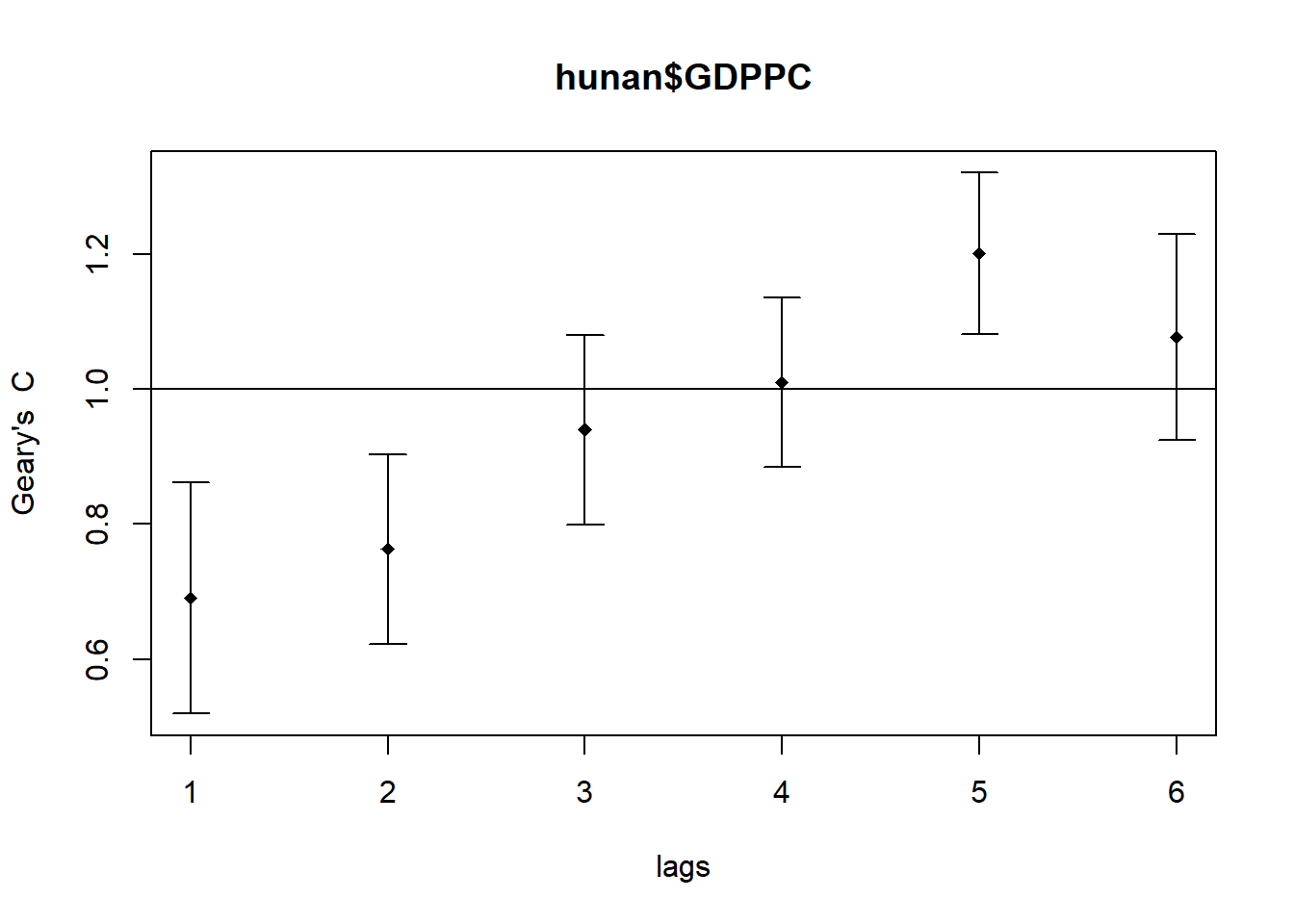
Compute Geary's C correlogram and plot

In the code chunk below, sp.correlogram() of spdep package is used to compute a 6-lag spatial correlogram of GDPPC. The global spatial autocorrelation used in Geary's C. The plot() of base Graph is then used to plot the output.

GC_corr <- sp.correlogram(wm_q, 
                          hunan$GDPPC, 
                          order=6, 
                          method="C", 
                          style="W")
plot(GC_corr)